
5 The Alkire-Foster Counting Methodology
This chapter provides a systematic overview of the multidimensional measurement methodology of Alkire and Foster (2007, 2011a), with an emphasis on the first measure of that class: the Adjusted Headcount Ratio or ![]() . It builds on previous chapters, which demonstrated the importance of adopting a multidimensional approach (Chapter 1), introduced the general framework (Chapter 2), and reviewed the different alternative methods for multidimensional measurement and analysis (Chapter 3). Chapter 3 also highlighted the advantages of certain axiomatic measures that consider the joint distribution of deprivations and exhibit a transparent and predictable behaviour with respect to different types of transformations. The fourth chapter reviewed counting methods to identify the poor (Chapter 4), which are frequently used in axiomatic measures.
. It builds on previous chapters, which demonstrated the importance of adopting a multidimensional approach (Chapter 1), introduced the general framework (Chapter 2), and reviewed the different alternative methods for multidimensional measurement and analysis (Chapter 3). Chapter 3 also highlighted the advantages of certain axiomatic measures that consider the joint distribution of deprivations and exhibit a transparent and predictable behaviour with respect to different types of transformations. The fourth chapter reviewed counting methods to identify the poor (Chapter 4), which are frequently used in axiomatic measures.
Why focus on the AF methodology and on ![]() in particular? As argued in 1.3, we focus on the AF methodology for a number of technical and practical reasons. From a technical perspective, being an axiomatic family of measures, the AF measures satisfy a number of desirable properties introduced in section 2.5, detailed in this chapter. From a practical perspective, the AF family of measures uses the intuitive counting approach to identify the poor, and explicitly considers the joint distribution of deprivations. Among the AF measures, the
in particular? As argued in 1.3, we focus on the AF methodology for a number of technical and practical reasons. From a technical perspective, being an axiomatic family of measures, the AF measures satisfy a number of desirable properties introduced in section 2.5, detailed in this chapter. From a practical perspective, the AF family of measures uses the intuitive counting approach to identify the poor, and explicitly considers the joint distribution of deprivations. Among the AF measures, the ![]() measure is particularly applicable due to its ability to use ordinal or binary data rigorously and because the measure and its consistent partial indices are intuitive. The technical and practical advantages of
measure is particularly applicable due to its ability to use ordinal or binary data rigorously and because the measure and its consistent partial indices are intuitive. The technical and practical advantages of ![]() make it a particularly attractive option to inform policy.
make it a particularly attractive option to inform policy.
It is worth noting from the beginning that the AF methodology is a general framework for measuring multidimensional poverty, although it is also suitable for measuring other phenomena (Alkire and Santos 2013). With the AF method, many key decisions are left to the user. These include the selection of the measure’s purpose, space, unit of analysis, dimensions, deprivation cutoffs (to determine when a person is deprived in a dimension), weights or values (to indicate the relative importance of the different deprivations), and poverty cutoff (to determine when a person has enough deprivations to be considered poor). This flexibility enables the methodology to have many diverse applications. The design of particular measures—which entail value judgements—is the subject of Chapter 6.
As described in section 2.2.2, the methodology for measuring multidimensional poverty consists of an identification and an aggregation method (Sen 1976). This chapter first describes how the AF methodology identifies people as poor using a ‘dual-cutoff’ counting method, standing on the shoulders of a long tradition of counting approaches that have been used in policy making (Chapter 4). The aggregation method builds on the unidimensional axiomatic poverty measures and directly extends the Foster–Greer–Thorbecke (1984) class of poverty measures introduced in section 2.1. The main focus of this chapter is the Adjusted Headcount Ratio ![]() , which reflects the incidence of poverty and the intensity of poverty, capturing the joint distribution of deprivations. The chapter shows how to ‘drill down’ into
, which reflects the incidence of poverty and the intensity of poverty, capturing the joint distribution of deprivations. The chapter shows how to ‘drill down’ into ![]() in order to unfold the distinctive partial indices that reveal the intuition and layers of information embedded in the summary measure, such as poverty at subgroup levels and its composition by dimension. Examples illustrate the methodology and also present standard tables and graphics that are used to convey results.
in order to unfold the distinctive partial indices that reveal the intuition and layers of information embedded in the summary measure, such as poverty at subgroup levels and its composition by dimension. Examples illustrate the methodology and also present standard tables and graphics that are used to convey results.
This chapter proceeds as follows. Section 5.1 presents the overview and practicality of the AF class of poverty measures, focusing especially on the Adjusted Headcount Ratio. Section 5.2 sets out the identification of who is poor using the dual-cutoff approach. Section 5.3 outlines the aggregation method used to construct the Adjusted Headcount Ratio. Section 5.4 presents the main distinctive characteristics of the Adjusted Headcount Ratio and section 5.5 presents its useful, consistent partial indices or components. We present a case study of the Adjusted Headcount Ratio using the global Multidimensional Poverty Index in section 5.6. Section 5.7 presents the members of the AF class of measures that can be constructed in the less common situations where data are cardinal, along with their properties and partial indices. Finally, section 5.8 reviews some empirical applications of the AF methology.
5.1 The AF Class of Poverty Measures: Overview and Practicality
The AF methodology of multidimensional poverty measurement creates a class of measures that both draws on the counting approach and extends the FGT class of measures in natural ways. Before proceeding with a more formal description of the AF methodology, we first provide a stepwise synthetic and intuitive presentation of how to obtain the Adjusted Headcount Ratio (![]() ), which is our focal measure. We also introduce the Adjusted Poverty Gap (
), which is our focal measure. We also introduce the Adjusted Poverty Gap (![]() ) and the Adjusted Squared Poverty Gap (or FGT) Measure (
) and the Adjusted Squared Poverty Gap (or FGT) Measure (![]() ). For clarity, we distinguish the steps that belong to the identification step and those that belong to the aggregation step.
). For clarity, we distinguish the steps that belong to the identification step and those that belong to the aggregation step.
One constructs these ![]() measures as follows:
measures as follows:
Identification
- Defining the set of indicators which will be considered in the multidimensional measure. Data for all indicators need to be available for the same person.
- Setting the deprivation cutoffs for each indicator, namely the level of achievement considered sufficient (normatively) in order to be non-deprived in each indicator.
- Applying the cutoffs to ascertain whether each person is deprived or not in each indicator.
- Selecting the relative weight or value that each indicator has, such that these sum to one.[1]
- Creating the weighted sum of deprivations for each person, which can be called his or her ‘deprivation score’.
- Determining (normatively) the poverty cutoff, namely, the proportion of weighted deprivations a person needs to experience in order to be considered multidimensionally poor, and identifying each person as multidimensionally poor or not according to the selected poverty cutoff.
Aggregation
- Computing the proportion of people who have been identified as multidimensionally poor in the population. This is the headcount ratio of multidimensional poverty
 , also called the incidence of multidimensional poverty.
 - Computing the average share of weighted indicators in which poor people are deprived. This entails adding up the deprivation scores of the poor and dividing them by the total number of poor people. This is the intensity of multidimensional poverty
 , also sometimes called the breadth of poverty.
 - Computing the
 measure as the product of the two previous partial indices:
  . Analogously, can be obtained as the mean of the vector of deprivation scores, which is also the sum of the weighted deprivations that poor people experience, divided by the total population.
When all indicators are ratio scale, one may also compute ![]() and
and ![]() as follows:
as follows:
- Computing the average poverty gap across all instances in which poor persons are deprived,
 . This entails computing the normalized deprivation gap as defined in equation (2.2): (
 ) for each person and indicator. The normalized gap is the difference between the deprivation cutoff and the poor person’s achievement for each indicator, divided by its deprivation cutoff. If a person’s achievement does not fall short of the deprivation cutoff, the normalized gap is zero. The average poverty gap is the mean of poor people’s weighted normalized deprivation gaps in those dimensions in which poor people are deprived and is one of the partial indices. This depth of multidimensional poverty is denoted by .
 - Computing the
 measure as the product of three partial indices:
  . Analogously, can be obtained as the sum of the weighted deprivation gaps that poor people experience, divided by the total population.
 - Computing the average severity of deprivation across all instances in which poor persons are deprived,
 . This entails computing the squared deprivation gap, that is, squaring each normalized gap computed in step 10. The average severity of deprivation is the mean of poor people’s weighted squared deprivation gaps in those dimensions in which they are deprived. This is the severity of multidimensional poverty, .
 - Computing the
 measure as the product of the following partial indices:
  . Analogously, can be obtained as the sum of the weighted squared deprivation gaps that poor people experience, divided by the total population.
Note that in all three cases (![]() ,
, ![]() and
and ![]() the deprivations experienced by people who have not been identified as poor (i.e. those whose deprivation score is below the poverty cutoff) are censored, hence not included; this censoring of the deprivations of the non-poor is consistent with the property of ‘poverty focus’ which—analogous to the unidimensional case—requires a poverty measure to be independent of the achievements of the non-poor. For further discussion see Alkire and Foster (2011a).
the deprivations experienced by people who have not been identified as poor (i.e. those whose deprivation score is below the poverty cutoff) are censored, hence not included; this censoring of the deprivations of the non-poor is consistent with the property of ‘poverty focus’ which—analogous to the unidimensional case—requires a poverty measure to be independent of the achievements of the non-poor. For further discussion see Alkire and Foster (2011a).
These three measures of the AF family, as well as any other member, satisfy many of the desirable properties introduced in section 2.5. Several properties are key for policy. The first is decomposability, which allows the index to be broken down by population subgroup (such as region or ethnicity) to show the characteristics of multidimensional poverty for each group. All AF measures satisfy population subgroup decomposability. So the poverty level of a society—as measured by any ![]() —is equivalent to the population-weighted sum of subgroup poverty levels, where subgroups are mutually exclusive and collectively exhaustive of the population.
—is equivalent to the population-weighted sum of subgroup poverty levels, where subgroups are mutually exclusive and collectively exhaustive of the population.
All AF measures can also be unpacked to reveal the dimensional deprivations contributing the most to poverty for any given group. This second key property—post-identification dimensional breakdown (section 2.2.4) — is not available with the standard headcount ratio and is particularly useful for policy.
The AF measures also satisfy dimensional monotonicity, meaning that whenever a poor person ceases to be deprived in a dimension, poverty decreases. The headcount ratio does not satisfy this. Dimensional monotonicity and breakdown both use the partial index of intensity.
A few comments on the AF class before we turn to the final key property for policy. All AF measures also have intuitive interpretations. The Adjusted Headcount Ratio![]() reflects the proportion of weighted deprivations the poor experience in a society out of the total number of deprivations this society could experience if all people were poor and were deprived in all dimensions. The Adjusted Poverty Gap
reflects the proportion of weighted deprivations the poor experience in a society out of the total number of deprivations this society could experience if all people were poor and were deprived in all dimensions. The Adjusted Poverty Gap![]() reflects the average weighted deprivation gap experienced by the poor out of the total number of deprivations this society could experience. The Adjusted Squared Poverty Gap Measure
reflects the average weighted deprivation gap experienced by the poor out of the total number of deprivations this society could experience. The Adjusted Squared Poverty Gap Measure ![]() reflects the average weighted squared gap or poverty severity experienced by the poor out of the total number of deprivations this society could experience. In all cases, the term ‘adjusted’ refers to the fact that all measures incorporate the intensity of multidimensional poverty—which is key to their properties.
reflects the average weighted squared gap or poverty severity experienced by the poor out of the total number of deprivations this society could experience. In all cases, the term ‘adjusted’ refers to the fact that all measures incorporate the intensity of multidimensional poverty—which is key to their properties.
Additionally, while each AF measure offers a summary statistic of multidimensional poverty, they are related to a set of consistent and intuitive partial indices, namely, poverty incidence (![]() ), intensity (
), intensity (![]() ), and a set of subgroup poverty estimates and dimensional deprivation indices (which in the case of the
), and a set of subgroup poverty estimates and dimensional deprivation indices (which in the case of the ![]() measure are called censored headcount ratios) and their corresponding percent contributions. Each
measure are called censored headcount ratios) and their corresponding percent contributions. Each ![]() measure can be unfolded into an array of informative indices.
measure can be unfolded into an array of informative indices.
Among the AF class of measures, the ![]() measure is particularly important because it can be implemented with ordinal data. This is critical for real-world applications. It is relevant when poverty is viewed from the capability perspective, for example, since many key functionings are commonly measured using ordinal variables. The
measure is particularly important because it can be implemented with ordinal data. This is critical for real-world applications. It is relevant when poverty is viewed from the capability perspective, for example, since many key functionings are commonly measured using ordinal variables. The ![]() measure satisfies the ordinality property introduced in section 2.5.1. This means that for any monotonic transformation of the ordinal variable and associated cutoff, overall poverty as estimated by
measure satisfies the ordinality property introduced in section 2.5.1. This means that for any monotonic transformation of the ordinal variable and associated cutoff, overall poverty as estimated by ![]() will not change. Moreover,
will not change. Moreover, ![]() has a natural interpretation as a measure of ‘unfreedom’ and generates a partial ordering that lies between first- and second-order dominance (Chapter 6). Because of its intuitiveness and practicality, this book mainly focuses on
has a natural interpretation as a measure of ‘unfreedom’ and generates a partial ordering that lies between first- and second-order dominance (Chapter 6). Because of its intuitiveness and practicality, this book mainly focuses on ![]() .
.
The remaining sections present the AF method more precisely yet, we hope, intuitively.
5.2 Identification of the Poor: The Dual-Cutoff Approach
Poverty measurement requires some identification function, which determines whether each person is to be considered poor. The unidimensional form of identification, discussed in section 2.2.1, entails a host of assumptions that restrict its applicability in practice and its desirability in principle.[2] From the perspective of the capability approach, a key conceptual drawback of viewing multidimensional poverty through a unidimensional lens is the loss of information on dimension-specific shortfalls; indeed, aggregation before identification converts dimensional achievements into one another without regard to dimension-specific cutoffs. In situations where dimensions are intrinsically valued and dimensional deprivations are inherently undesirable, there are good reasons to look beyond a unidimensional approach to identification methods that focus on dimensional shortfalls.
In the multidimensional measurement setting, where there are multiple variables, identification is a substantially more challenging exercise. As explained in section 2.2.2, a variety of methods can be used for identification in multidimensional poverty measurement. Here we follow a censored achievement approach. This approach first requires determining who is deprived in each dimension by comparing the person’s achievement against the corresponding deprivation cutoff and thus considering only deprived achievements (and ignoring—or censoring—achievements above the deprivation cutoff) for the identification of the poor. One prominent method used within the censored achievement approach is the counting approach, which is precisely the identification approach followed in the AF methodology, among others (Chapter 4).
As we have seen, a counting approach first identifies whether a person is deprived or not in each dimension and then identifies a person as poor according to the number (count) of deprivations she experiences. Note that ‘number’ here has a broad meaning as dimensions may be weighted differently. As reviewed in Chapter 4, the use of a counting approach to identification in multidimensional poverty measurement is not new. However, the value added of the AF methodology is threefold. In the first place, the AF methodology has formalized the counting approach to identification into a dual-cutoff approach, clarifying the requirement of two distinct sets of thresholds to define poverty in the multidimensional context. One is the set of deprivation cutoffs, which identify whether a person is deprived with respect to each dimension. Then, a (single) poverty cutoff delineates how widely deprived a person must be in order to be considered poor.
Second, as a consequence of using a dual-cutoff approach, the AF methodology considers the joint distribution of deprivations at the identification step and not just at the aggregation step, as previous methodologies did (almost all non-counting methodologies used the union criterion). Third, the AF methodology has integrated the counting approach to identification with an aggregation methodology that extends the unidimensional FGT measures, overcoming the limitations of the headcount ratio (which most counting methods used) yet allowing intuitive interpretations.[3]
Thus the AF methodology draws together the counting traditions – widely known for their practicality and policy appeal – and the widely used FGT class of axiomatic measures in order to assess multidimensional poverty, and stands on the shoulders of both traditions.
5.2.1 The Deprivation Cutoffs: Identifying Deprivations and Obtaining Deprivation Scores
Bourguignon and Chakravarty (2003) contend that ‘a multidimensional approach to poverty defines poverty as a shortfall from a threshold on each dimension of an individual’s wellbeing’.[4] Following them and the plethora of counting methods reviewed in Chapter 4, the AF measures use a deprivation cutoff for each dimension, defined and applied as described in this section.
As introduced in section 2.2, the base information in multidimensional poverty measurement is typically represented by an ![]() dimensional achievement matrix
dimensional achievement matrix ![]() , where
, where ![]() is the achievement of person
is the achievement of person ![]() in dimension
in dimension ![]() . For simplicity, as done in section 2.2, it is assumed that achievements can be represented by non-negative real numbers (i.e.
. For simplicity, as done in section 2.2, it is assumed that achievements can be represented by non-negative real numbers (i.e. ![]() ) and that higher achievements are preferred to lower ones.
) and that higher achievements are preferred to lower ones.
For each dimension ![]() , a threshold
, a threshold ![]() is defined as the minimum achievement required in order to be non-deprived. This threshold is called a deprivation cutoff. Deprivation cutoffs are collected in the
is defined as the minimum achievement required in order to be non-deprived. This threshold is called a deprivation cutoff. Deprivation cutoffs are collected in the ![]() -dimensional vector
-dimensional vector ![]() . Given each person’s achievement in each dimension
. Given each person’s achievement in each dimension ![]() , if the ith person’s achievement level in a given dimension
, if the ith person’s achievement level in a given dimension ![]() falls short of the respective deprivation cutoff
falls short of the respective deprivation cutoff ![]() , the person is said to be deprived in that dimension (that is, if
, the person is said to be deprived in that dimension (that is, if ![]() ). If the person’s level is at least as great as the deprivation cutoff, the person is not deprived in that dimension.
). If the person’s level is at least as great as the deprivation cutoff, the person is not deprived in that dimension.
As Chapter 2 introduced, from the achievement matrix ![]() and the vector of deprivation cutoffs
and the vector of deprivation cutoffs ![]() , one can obtain a deprivation matrix
, one can obtain a deprivation matrix ![]() such that
such that ![]() whenever
whenever ![]() and
and ![]() , otherwise, for all
, otherwise, for all ![]() and for all
and for all ![]() . In other words, if person
. In other words, if person ![]() is deprived in dimension
is deprived in dimension ![]() , then the person is assigned a deprivation status value of 1, and 0 otherwise. The matrix
, then the person is assigned a deprivation status value of 1, and 0 otherwise. The matrix ![]() summarizes the deprivation status value of all people in all dimensions of matrix
summarizes the deprivation status value of all people in all dimensions of matrix ![]() . The vector
. The vector ![]() summarizes the deprivation status values of person
summarizes the deprivation status values of person ![]() in all dimensions, and the vector
in all dimensions, and the vector ![]() summarizes the deprivation status values of all persons in dimension
summarizes the deprivation status values of all persons in dimension ![]() .
.
The deprivation in each of the ![]() dimensions may not have the same relative importance. Thus, a vector
dimensions may not have the same relative importance. Thus, a vector ![]() of weights or deprivation values is used to indicate the relative importance of a deprivation in each dimension. The deprivation value attached to dimension
of weights or deprivation values is used to indicate the relative importance of a deprivation in each dimension. The deprivation value attached to dimension ![]() is denoted by
is denoted by ![]() . If each deprivation is viewed as having equal importance, then this is a benchmark ‘counting’ case. If deprivations are viewed as having different degrees of importance, general weights are applied using a weighting vector whose entries vary, with higher weights indicating greater relative value.
. If each deprivation is viewed as having equal importance, then this is a benchmark ‘counting’ case. If deprivations are viewed as having different degrees of importance, general weights are applied using a weighting vector whose entries vary, with higher weights indicating greater relative value.
Intricate weighting systems create challenges in interpretation, so it can be useful to choose the dimensions such that the natural weights among them are roughly equal or else to group dimensions into categories that have roughly equal weights (Atkinson 2003). The deprivation values affect identification because they determine the minimum combinations of deprivations that will identify a person as being poor. They also affect aggregation by altering the relative contributions of deprivations to overall poverty (for more on weights see Chapter 6). Yet importantly the deprivation values do not function as weights that govern trade-offs between dimensions for every possible combination of ratio-scale achievement levels, as they do in a traditional composite index. Because each deprivation status value is binary, the role of deprivation values differs from the role of weights in traditional composite indices.
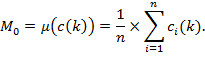
Based on the deprivation profile, each person is assigned a deprivation score that reflects the breadth of each person’s deprivations across all dimensions. The deprivation score of each person is the sum of her weighted deprivations. Formally, the deprivation score is given by ![]() . The score increases as the number of deprivations a person experiences increases, and reaches its maximum when the person is deprived in all dimensions. A person who is not deprived in any dimension has a deprivation score equal to 0. We denote the deprivation score of person
. The score increases as the number of deprivations a person experiences increases, and reaches its maximum when the person is deprived in all dimensions. A person who is not deprived in any dimension has a deprivation score equal to 0. We denote the deprivation score of person ![]() by
by ![]() and the column vector of deprivation scores for all persons by
and the column vector of deprivation scores for all persons by ![]() .
.
5.2.2 Alternative Notation and Presentation
Distinct notational presentations can be employed for the weights, deprivation scores, deprivation score vector, poverty cutoff, poverty measures, and partial indices. Substantively, alternative presentations are identical in that they each identify precisely the same persons as poor and generate the same poverty measure value and identical partial indices. What differ are the numerical values of weights, deprivation scores, and poverty cutoff. For didactic purposes we explain the main options so as to avoid confusion among researchers using different notational conventions.
Alternative notations arise from two decisions. The first decision is whether to define weights that sum to one, i.e. ![]() , or whether weights sum to the number of dimensions under consideration,
, or whether weights sum to the number of dimensions under consideration, ![]() . We refer to the first as normalized weights and to the second as non-normalized or numbered weights. The normalized weight of a dimension reflects the share (or percentage) of total weight given to a particular dimension. The deprivation score then shows the percentage of weighted dimensions in which a person is deprived and lies between 0 and 1. In the numbered case, deprivation scores range between 0 and
. We refer to the first as normalized weights and to the second as non-normalized or numbered weights. The normalized weight of a dimension reflects the share (or percentage) of total weight given to a particular dimension. The deprivation score then shows the percentage of weighted dimensions in which a person is deprived and lies between 0 and 1. In the numbered case, deprivation scores range between 0 and ![]() . If person
. If person ![]() is deprived in all dimensions, then
is deprived in all dimensions, then ![]() . Depending on the weighting structure, one of these options may be more intuitive than the other. For example, if dimensions are equally weighted, the deprivation count vector shows the number of dimensions in which each person is deprived. Thus, while in the normalized case one may state that a person is deprived in 43% of the weighted dimensions, in the non-normalized case one states that a person is deprived in three out of seven dimensions, which is more intuitive. However, if dimensions are not equally weighted, as is common in practice, normalized weights may be more intuitive. Suppose there are seven dimensions and a person is deprived in two dimensions having weights of 25% and 10%, respectively. Their numbered deprivation score would be 2.45 = (0.25*7 + 0.10*7). This same situation could be communicated more intuitively by saying that this person is deprived in 35% of the weighted dimensions.
. Depending on the weighting structure, one of these options may be more intuitive than the other. For example, if dimensions are equally weighted, the deprivation count vector shows the number of dimensions in which each person is deprived. Thus, while in the normalized case one may state that a person is deprived in 43% of the weighted dimensions, in the non-normalized case one states that a person is deprived in three out of seven dimensions, which is more intuitive. However, if dimensions are not equally weighted, as is common in practice, normalized weights may be more intuitive. Suppose there are seven dimensions and a person is deprived in two dimensions having weights of 25% and 10%, respectively. Their numbered deprivation score would be 2.45 = (0.25*7 + 0.10*7). This same situation could be communicated more intuitively by saying that this person is deprived in 35% of the weighted dimensions.
The second decision is whether to express the formulas using the deprivation matrix ![]() and the (explicitly separate) weighting vector
and the (explicitly separate) weighting vector ![]() in an explicit way, or whether to express them in terms of a weighted deprivation matrix denoted by
in an explicit way, or whether to express them in terms of a weighted deprivation matrix denoted by ![]() such that
such that ![]() if
if ![]() and
and ![]() if
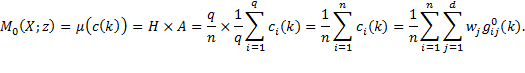
if ![]() . These two decisions lead to four possible—but totally equivalent—notations, as detailed in Box 5.7. This chapter, and most of this book, uses normalized weights and expresses formulas using the deprivation matrix and the weight vector. We refer to this as Method I. Method II uses normalized weights with the weighted deprivation matrix. Method III uses non-normalized weights and expresses formulas using the deprivation matrix and the weight vector. Methods II and III are not further discussed in this chapter, but all the formulas are stated in Box 5.7. Finally, Method IV uses non-normalized weights and expresses the formulas using the weighted deprivation matrix, aligned with the notation used in Alkire and Foster (2011a), which is presented in Box 5.3, Box 5.6, and Box 5.7. What is particularly elegant about Method IV is that the AF measures can be expressed as the mean of the relevant censored deprivation matrix, as we shall elaborate subsequently.
. These two decisions lead to four possible—but totally equivalent—notations, as detailed in Box 5.7. This chapter, and most of this book, uses normalized weights and expresses formulas using the deprivation matrix and the weight vector. We refer to this as Method I. Method II uses normalized weights with the weighted deprivation matrix. Method III uses non-normalized weights and expresses formulas using the deprivation matrix and the weight vector. Methods II and III are not further discussed in this chapter, but all the formulas are stated in Box 5.7. Finally, Method IV uses non-normalized weights and expresses the formulas using the weighted deprivation matrix, aligned with the notation used in Alkire and Foster (2011a), which is presented in Box 5.3, Box 5.6, and Box 5.7. What is particularly elegant about Method IV is that the AF measures can be expressed as the mean of the relevant censored deprivation matrix, as we shall elaborate subsequently.
5.2.3 The Second Cutoff: Identifying the Poor
In addition to the deprivation cutoffs ![]() , the AF methodology uses a second cutoff or threshold to identify the multidimensionally poor. This is called the poverty cutoff and is denoted by
, the AF methodology uses a second cutoff or threshold to identify the multidimensionally poor. This is called the poverty cutoff and is denoted by ![]() . The poverty cutoff is the minimum deprivation score a person needs to exhibit in order to be identified as poor. This poverty cutoff is implemented using an identification function
. The poverty cutoff is the minimum deprivation score a person needs to exhibit in order to be identified as poor. This poverty cutoff is implemented using an identification function ![]() , which depends upon each person’s achievement vector
, which depends upon each person’s achievement vector ![]() the deprivation cutoff vector
the deprivation cutoff vector ![]() , the weight vector
, the weight vector ![]() , and the poverty cutoff
, and the poverty cutoff ![]() . If the person is poor, the identification function takes on a value of 1; if the person is not poor, the identification function has a value of 0. Notationally, the identification function is defined as
. If the person is poor, the identification function takes on a value of 1; if the person is not poor, the identification function has a value of 0. Notationally, the identification function is defined as ![]() if
if![]() and
and ![]() otherwise. In other words,
otherwise. In other words, ![]() identifies person
identifies person ![]() as poor when his or her deprivation score is at least
as poor when his or her deprivation score is at least ![]() ; if the deprivation score falls below the cutoff
; if the deprivation score falls below the cutoff ![]() , then person
, then person ![]() is not poor according to
is not poor according to ![]() . Since
. Since ![]() is dependent on both the set of within-dimension deprivation cutoffs
is dependent on both the set of within-dimension deprivation cutoffs ![]() and the across-dimension cutoff
and the across-dimension cutoff ![]() ,
, ![]() is referred to as the dual cutoff method of identification, or sometimes as the ‘intermediary’ method.
is referred to as the dual cutoff method of identification, or sometimes as the ‘intermediary’ method.
Within the counting approach to identification, the most commonly used multidimensional identification strategy is the union criterion.[5] Most of the poverty indices discussed in Chapter 3 use the union criterion, by which a person ![]() is identified as multidimensionally poor if she is deprived in at least one dimension (
is identified as multidimensionally poor if she is deprived in at least one dimension (![]() ). At the other extreme, another identification criterion is the intersection criterion, which identifies person
). At the other extreme, another identification criterion is the intersection criterion, which identifies person ![]() as being poor only if she is deprived in all dimensions (
as being poor only if she is deprived in all dimensions (![]() ). Both these approaches have the advantage of identifying the same people as poor regardless of the relative weights set on the dimensions. But the identification of who is poor in each case is exceedingly sensitive to the choice of dimensions. Also these strategies can be too imprecise for policy: in many applications, a union identification identifies a very large proportion of the population as poor, whereas an intersection approach identifies a vanishingly small number of people as poor. A natural middle-ground alternative is to use an intermediate cutoff level for
). Both these approaches have the advantage of identifying the same people as poor regardless of the relative weights set on the dimensions. But the identification of who is poor in each case is exceedingly sensitive to the choice of dimensions. Also these strategies can be too imprecise for policy: in many applications, a union identification identifies a very large proportion of the population as poor, whereas an intersection approach identifies a vanishingly small number of people as poor. A natural middle-ground alternative is to use an intermediate cutoff level for ![]() that lies somewhere between the two extremes of union and intersection.
that lies somewhere between the two extremes of union and intersection.
The AF dual-cutoff identification strategy provides an overarching framework that includes the two extremes of union and intersection criteria and also the range of intermediate possibilities.[6] Notice that ![]() includes the union and intersection methods as special cases. In the case of union, the poverty cutoff is less than or equal to the dimension with the lowest weight:
includes the union and intersection methods as special cases. In the case of union, the poverty cutoff is less than or equal to the dimension with the lowest weight: ![]() Whereas in the case of intersection, the poverty cutoff takes its highest possible value of
Whereas in the case of intersection, the poverty cutoff takes its highest possible value of ![]() . In Box 5.1, we present different identification strategies using an example.
. In Box 5.1, we present different identification strategies using an example.
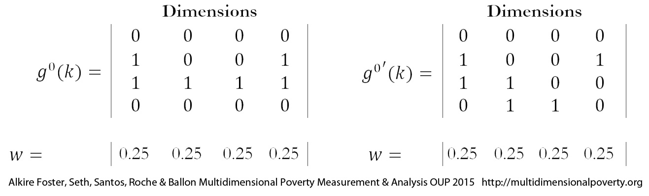
Box 5.1 Different Identification Strategies: Union, Intersection, and Intermediate Cutoff
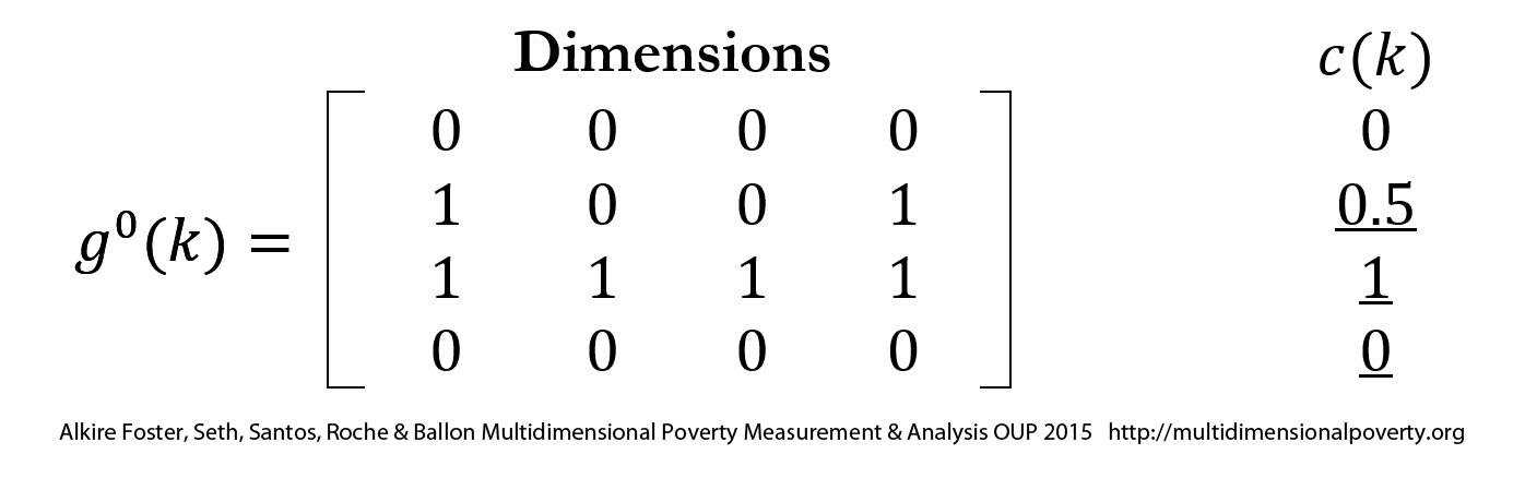
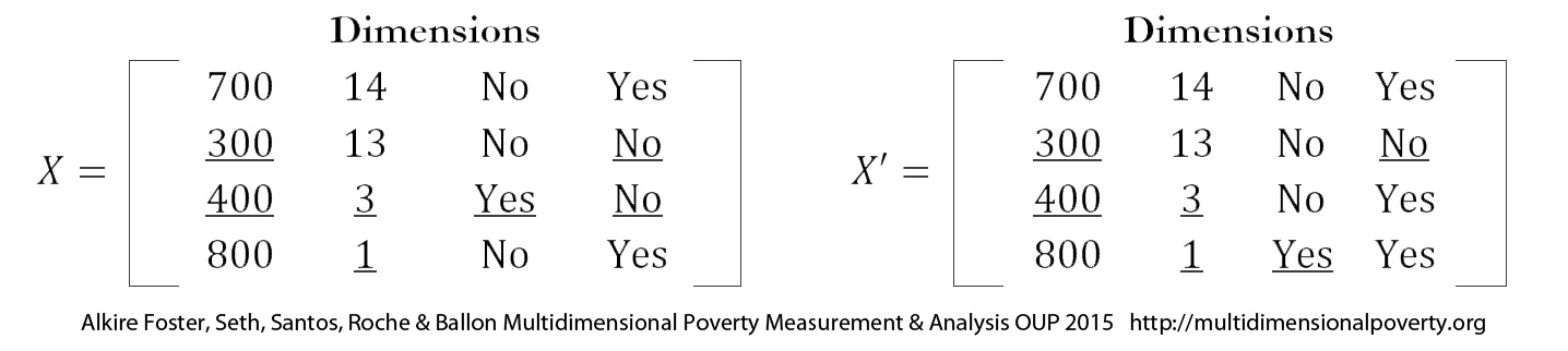
Suppose there is a hypothetical society containing four persons and multidimensional poverty is analysed using four dimensions: standard of living as measured by income, level of knowledge as measured by years of education, nutritional status as measured by Body Mass Index (BMI), and access to public services as measured by access to electricity. The ![]() matrix
matrix ![]() contains the achievements of four persons in four dimensions.
contains the achievements of four persons in four dimensions.
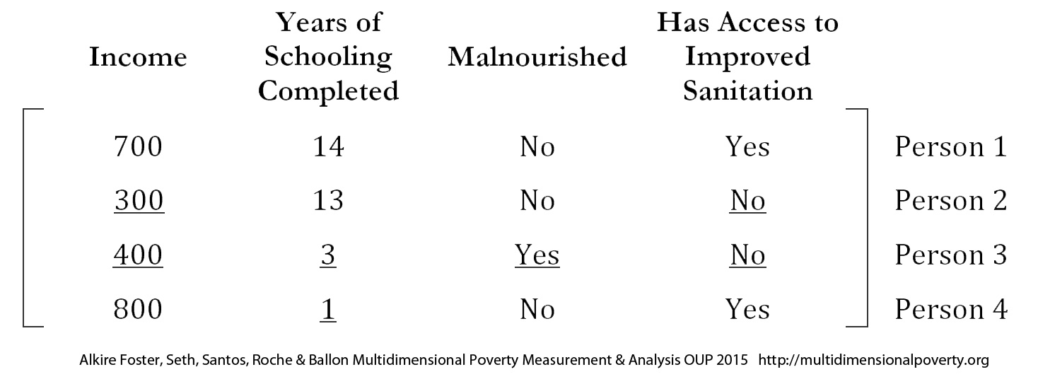
For example, the income of Person 3 is 400 Units; whereas Person 4’s is 800 Units. Person 1 has completed fourteen years of schooling; whereas Person 2 has completed thirteen years of schooling. Person 3 is the only person who is malnourished of all four persons. Two persons in our example have access to improved sanitation. Thus, each row of matrix ![]() contains the achievements of each person in four dimensions, whereas each column of the matrix contains the achievements of four persons in each of the four dimensions. All dimensions are equally weighted and thus the weight vector is
contains the achievements of each person in four dimensions, whereas each column of the matrix contains the achievements of four persons in each of the four dimensions. All dimensions are equally weighted and thus the weight vector is ![]() . The deprivation cutoff vector is denoted by
. The deprivation cutoff vector is denoted by ![]() (500, 5, Not malnourished, Has access to improved sanitation), which is used to identify who is deprived in each dimension. The achievement matrix
(500, 5, Not malnourished, Has access to improved sanitation), which is used to identify who is deprived in each dimension. The achievement matrix ![]() has three persons who are deprived (see the underlined entries) in one or more dimensions. Person 1 has no deprivation at all.
has three persons who are deprived (see the underlined entries) in one or more dimensions. Person 1 has no deprivation at all.
Based on the deprivation status, we construct the deprivation matrix ![]() , where a deprivation status score of 1 is assigned if a person is deprived in a dimension and a status score of 0 is given otherwise.
, where a deprivation status score of 1 is assigned if a person is deprived in a dimension and a status score of 0 is given otherwise.
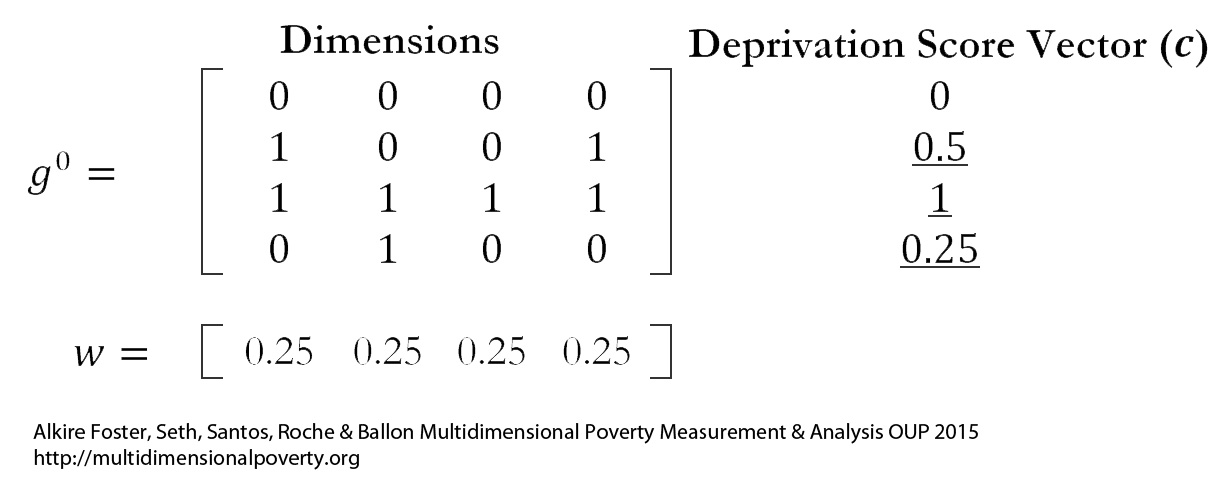
The weighted sum of these status scores is the deprivation score (![]() ) of each person. For example, the first person has no deprivation and so the deprivation score is 0, whereas the third person is deprived in all dimensions and thus has the highest deprivation score of 1. Similarly, the deprivation score of the second person is
) of each person. For example, the first person has no deprivation and so the deprivation score is 0, whereas the third person is deprived in all dimensions and thus has the highest deprivation score of 1. Similarly, the deprivation score of the second person is ![]() (
(![]() ). The union identification strategy identifies a person as poor if the person is identified as deprived in any of the four dimensions. In that case, three of the four persons are identified as poor. On the other hand, an intersection identification strategy requires that a person is identified as poor if the person is deprived in all dimensions. In that case, only one of four persons is identified as poor in this case. An intermediate approach sets a cutoff between union and intersection, say,
). The union identification strategy identifies a person as poor if the person is identified as deprived in any of the four dimensions. In that case, three of the four persons are identified as poor. On the other hand, an intersection identification strategy requires that a person is identified as poor if the person is deprived in all dimensions. In that case, only one of four persons is identified as poor in this case. An intermediate approach sets a cutoff between union and intersection, say, ![]() , which is equivalent to being deprived in two of four equally weighted dimensions. This strategy identifies a person as poor if the person is deprived in half or more of weighted dimensions, which in this case means that two of the four persons are identified as poor.
, which is equivalent to being deprived in two of four equally weighted dimensions. This strategy identifies a person as poor if the person is deprived in half or more of weighted dimensions, which in this case means that two of the four persons are identified as poor.
The dual-cutoff identification strategy has a number of characteristics that deserve mention. First, it is ‘poverty focused’ in that an increase in an achievement level ![]() of a non-poor person leaves its value unchanged. Second, it is ‘deprivation focused’ in that an increase in any non-deprived achievement
of a non-poor person leaves its value unchanged. Second, it is ‘deprivation focused’ in that an increase in any non-deprived achievement ![]() leaves the value of the identification function unchanged; in other words, a person’s poverty status is not affected by changes in the levels of non-deprived achievements. This latter property separates
leaves the value of the identification function unchanged; in other words, a person’s poverty status is not affected by changes in the levels of non-deprived achievements. This latter property separates ![]() from the ‘aggregate achievement’ approach which allows a higher level of achievement to compensate for lower levels of achievement in other dimensions. Finally, the dual-cutoff identification method can be meaningfully used with ordinal data, since a person’s poverty status is unchanged when an admissible transformation is applied to an achievement level and its associated cutoff.
from the ‘aggregate achievement’ approach which allows a higher level of achievement to compensate for lower levels of achievement in other dimensions. Finally, the dual-cutoff identification method can be meaningfully used with ordinal data, since a person’s poverty status is unchanged when an admissible transformation is applied to an achievement level and its associated cutoff.
5.2.4 Dual-Cutoff Approach and Censoring
The transition between the identification step and the aggregation step is most easily understood by examining a progression of matrices. There are two kinds of censoring, each of which follows the application of the two kinds of cutoffs: deprivation and poverty. By applying the deprivation cutoffs to the achievement matrix ![]() , we constructed the deprivation matrix
, we constructed the deprivation matrix ![]() replacing each entry in
replacing each entry in ![]() that is below its respective deprivation cutoff
that is below its respective deprivation cutoff ![]() with 1 and each entry that is not below its deprivation cutoff with 0. This is the first censoring, because the achievements above their corresponding deprivation cutoff are converted into 0. The deprivation matrix provides a snapshot of who is deprived in which dimension.
with 1 and each entry that is not below its deprivation cutoff with 0. This is the first censoring, because the achievements above their corresponding deprivation cutoff are converted into 0. The deprivation matrix provides a snapshot of who is deprived in which dimension.
Next, the poor are identified by applying the poverty cutoff ![]() and thus a new matrix can be obtained from the deprivation matrix: the censored deprivation matrix, which is denoted by
and thus a new matrix can be obtained from the deprivation matrix: the censored deprivation matrix, which is denoted by ![]() . Each element in
. Each element in ![]() is obtained by multiplying the corresponding element in
is obtained by multiplying the corresponding element in ![]() by the identification function
by the identification function ![]() . Formally,
. Formally, ![]() for all
for all ![]() and for all
and for all ![]() . What does this do? If person
. What does this do? If person ![]() is poor and thus
is poor and thus ![]() , then the person’s deprivation status in every dimension remains unchanged and so does the row containing the deprivation information of the person. If person
, then the person’s deprivation status in every dimension remains unchanged and so does the row containing the deprivation information of the person. If person ![]() is not poor and thus
is not poor and thus ![]() , then their deprivation status in every dimension becomes 0, which is equivalent to censoring the deprivations of persons who are not poor. This second censoring step is key to the AF methodology. As we will see in subsequent sections, the censored deprivation matrices embody the identification step and are the basic constructs used in the aggregation step.
, then their deprivation status in every dimension becomes 0, which is equivalent to censoring the deprivations of persons who are not poor. This second censoring step is key to the AF methodology. As we will see in subsequent sections, the censored deprivation matrices embody the identification step and are the basic constructs used in the aggregation step.
From the censored deprivation matrix, a censored deprivation score can be obtained. This applies the identification function to the original deprivation score vector used to identify the poor. The censored deprivation score of person ![]() is denoted by
is denoted by ![]() , and can be obtained as
, and can be obtained as ![]() . The censored deprivation score vector is denoted by
. The censored deprivation score vector is denoted by ![]() . Note that by definition,
. Note that by definition, ![]() has been censored of all deprivations that are less than the value of
has been censored of all deprivations that are less than the value of ![]() . Thus, when
. Thus, when ![]() , then
, then ![]() (deprivation score of the person), but if
(deprivation score of the person), but if ![]() , then
, then ![]() .[7]
.[7]
Note that there is one case where the second censoring is not relevant: when the poverty cutoff ![]() corresponds to the union approach, then any person who is deprived in any dimension is considered poor and the censored and original matrices are identical.
corresponds to the union approach, then any person who is deprived in any dimension is considered poor and the censored and original matrices are identical.
Although the censored matrices are used to construct multidimensional poverty measures, the original deprivation matrix still provides useful information, as we shall see later in constructing ‘raw’ or uncensored deprivation headcount ratios by dimension and analysing their change over time.
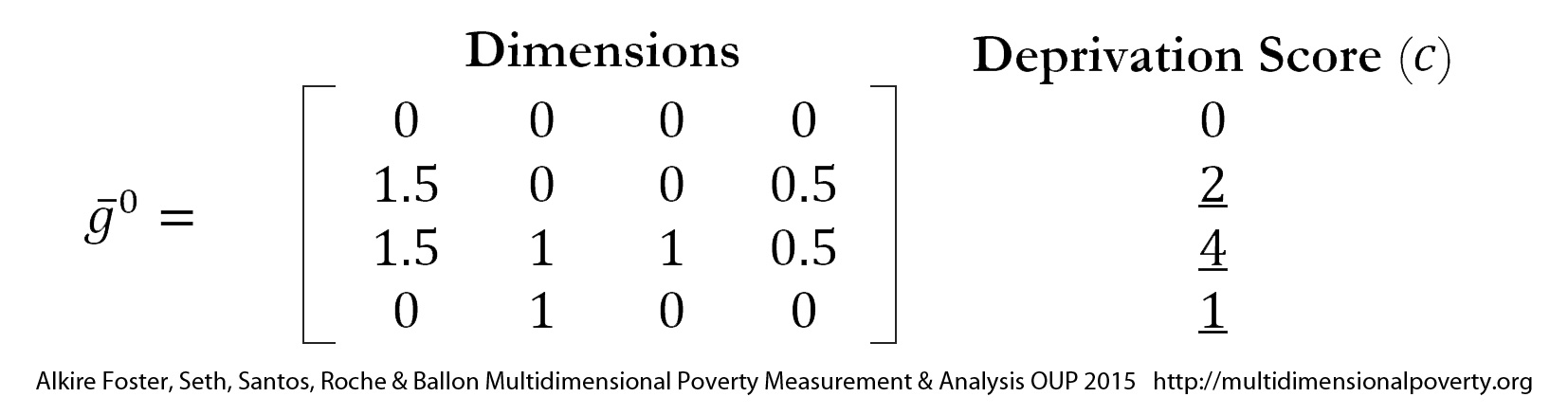
Before moving on to the aggregation step to create the Adjusted Headcount Ratio, let us provide an example of how to obtain the censored deprivation score vector from an achievement matrix in Box 5.2.
Box 5.2 Obtaining the Censored Deprivation Score Vector from an Achievement Matrix
Consider the ![]() achievement matrix
achievement matrix ![]() and the deprivation cutoff vector
and the deprivation cutoff vector ![]() in Box 5.1. As earlier, each of the four dimensions receives a weight equal to 0.25 and weights sum to one. Assume in this case that a person is identified as poor if deprived in half or more of the four equally weighted dimensions, i.e.
in Box 5.1. As earlier, each of the four dimensions receives a weight equal to 0.25 and weights sum to one. Assume in this case that a person is identified as poor if deprived in half or more of the four equally weighted dimensions, i.e. ![]() .
.
The achievement matrix ![]() has three persons who are deprived in one or more dimensions. Based on the deprivation status, a deprivation matrix
has three persons who are deprived in one or more dimensions. Based on the deprivation status, a deprivation matrix ![]() is constructed in which a deprivation status score of 1 is assigned if a person is deprived in a dimension and a status score of 0 is given otherwise. The weighted sum of these status scores yields the deprivation score of each person
is constructed in which a deprivation status score of 1 is assigned if a person is deprived in a dimension and a status score of 0 is given otherwise. The weighted sum of these status scores yields the deprivation score of each person ![]() .
.
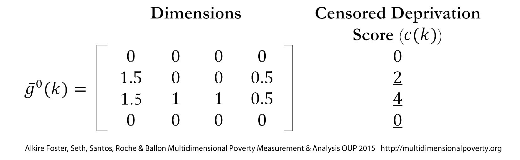
Note that two persons (second and third) have deprivation scores that are greater than or equal to 0.5. They are considered to be poor (![]() ), and hence their entries in the censored deprivation matrix are the same as in the deprivation matrix. However, the fourth person has a single deprivation and hence is not poor. This single deprivation is censored in the censored deprivation matrix, which only displays the deprivations of the poor, as depicted below.[8]
), and hence their entries in the censored deprivation matrix are the same as in the deprivation matrix. However, the fourth person has a single deprivation and hence is not poor. This single deprivation is censored in the censored deprivation matrix, which only displays the deprivations of the poor, as depicted below.[8]

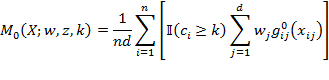
5.3 Aggregation: The Adjusted Headcount Ratio
The aggregation step of our methodology builds upon the FGT class of unidimensional poverty measures and likewise generates a parametric class of measures. Just as each FGT measure can be viewed as the mean of an appropriate vector built from the original data and censored using the poverty line, the Adjusted Headcount Ratio is the mean of the censored deprivation score vector:
|
|
(5.1) |
This section elaborates the Adjusted Headcount Ratio; the other measures in the AF class are presented in section 5.7.
A second way of viewing ![]() is in terms of partial indices—measures that provide basic information on a single aspect of poverty. The Adjusted Headcount Ratio, denoted as
is in terms of partial indices—measures that provide basic information on a single aspect of poverty. The Adjusted Headcount Ratio, denoted as ![]() , can also be written as the product of two partial indices. The first partial index
, can also be written as the product of two partial indices. The first partial index ![]() is the percentage of the population that is poor or the multidimensional headcount ratio or the incidence of poverty. The second index
is the percentage of the population that is poor or the multidimensional headcount ratio or the incidence of poverty. The second index ![]() is the intensity of poverty.
is the intensity of poverty.
|
|
(5.2) |
|
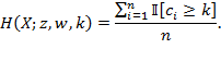
The headcount ratio or poverty incidence ![]() is the proportion of the population that is poor. It is defined as
is the proportion of the population that is poor. It is defined as ![]() , where
, where ![]() is number of persons identified as poor using the dual-cutoff approach.[9]
is number of persons identified as poor using the dual-cutoff approach.[9]
In turn, poverty intensity ![]() is the average deprivation score across the poor. Notice that the censored deprivation score
is the average deprivation score across the poor. Notice that the censored deprivation score ![]() represents the share of possible deprivations experienced by a poor person
represents the share of possible deprivations experienced by a poor person ![]() . So the average deprivation score across the poor is given by
. So the average deprivation score across the poor is given by ![]() . Like the poverty gap information in income poverty, this partial index conveys relevant information about multidimensional poverty, in that persons who experience simultaneous deprivations in a higher fraction of dimensions have a higher intensity of poverty and are poorer than others having a lower intensity.
. Like the poverty gap information in income poverty, this partial index conveys relevant information about multidimensional poverty, in that persons who experience simultaneous deprivations in a higher fraction of dimensions have a higher intensity of poverty and are poorer than others having a lower intensity.
Thus, ![]() is given by
is given by
As a simple product of the two partial indices ![]() and
and ![]() , the measure
, the measure ![]() is sensitive to the incidence and the intensity of multidimensional poverty. It clearly satisfies dimensional monotonicity, since if a poor person becomes deprived in an additional dimension, then
is sensitive to the incidence and the intensity of multidimensional poverty. It clearly satisfies dimensional monotonicity, since if a poor person becomes deprived in an additional dimension, then ![]() rises and so does
rises and so does ![]() . Another interpretation of
. Another interpretation of ![]() is that it provides the share of weighted deprivations experienced by the poor divided by the maximum possible deprivations that could possibly be experienced if all people were poor and were deprived in all dimensions.
is that it provides the share of weighted deprivations experienced by the poor divided by the maximum possible deprivations that could possibly be experienced if all people were poor and were deprived in all dimensions.
Let us provide an example using the same censored deprivation matrix and the censored deprivation score vector as in Box 5.2.
The headcount ratio ![]() is the proportion of people who are poor, which is two out of four persons in the above matrix. The intensity
is the proportion of people who are poor, which is two out of four persons in the above matrix. The intensity ![]() is the average deprivation share among the poor, which in this example is the average of
is the average deprivation share among the poor, which in this example is the average of ![]() and
and ![]() , i.e. equal to
, i.e. equal to ![]() . It is easy to see that the multidimensional headcount ratio
. It is easy to see that the multidimensional headcount ratio ![]() . In this example
. In this example ![]()
![]() and
and ![]() , so
, so ![]() . It is straightforward to verify that
. It is straightforward to verify that ![]() is the average of all elements in the censored deprivation score vector
is the average of all elements in the censored deprivation score vector ![]() , i.e.
, i.e. ![]() . Analogously, it is equivalent to compute
. Analogously, it is equivalent to compute ![]() as the weighted sum of deprivation status values divided by the total number of people:
as the weighted sum of deprivation status values divided by the total number of people: ![]() .
.
We have outlined the different expressions in terms of normalized weights (Method I in Box 5.7). Let us provide an alternative approach for computing the Adjusted Headcount Ratio when the weights are non-normalized such that ![]() , i.e. adding to the total number of dimensions, following the notation presented in Alkire and Foster (2011a). In order to do so, we need to introduce the weighted deprivation matrix. From the deprivation matrix, a weighted deprivation matrix can be constructed by replacing the deprivation status value of a deprived person with the value or weight assigned to the corresponding dimension. Formally, we denote the weighted deprivation matrix by
, i.e. adding to the total number of dimensions, following the notation presented in Alkire and Foster (2011a). In order to do so, we need to introduce the weighted deprivation matrix. From the deprivation matrix, a weighted deprivation matrix can be constructed by replacing the deprivation status value of a deprived person with the value or weight assigned to the corresponding dimension. Formally, we denote the weighted deprivation matrix by ![]() such that
such that ![]() if
if ![]() and
and ![]() if
if ![]() . Like the censored deprivation matrix, the censored weighted deprivation matrix
. Like the censored deprivation matrix, the censored weighted deprivation matrix ![]() can be constructed such that
can be constructed such that ![]() for all
for all ![]() and all
and all ![]() . From the weighted deprivation matrix
. From the weighted deprivation matrix ![]() , the Adjusted Headcount Ratio can be defined as
, the Adjusted Headcount Ratio can be defined as
|
|
That is, ![]() is the mean of the weighted censored deprivation matrix. Thus, the Adjusted Headcount Ratio is the sum of the weighted censored deprivation status values of the poor or
is the mean of the weighted censored deprivation matrix. Thus, the Adjusted Headcount Ratio is the sum of the weighted censored deprivation status values of the poor or ![]() divided by the highest possible sum of weighted deprivation status values, or
divided by the highest possible sum of weighted deprivation status values, or ![]() .
.
Let us provide an example and show how the Adjusted Headcount Ratio is computed using this approach. Recall this deprivation matrix in Box 5.1. In this example, suppose the dimensions are unequally weighted and the weight vector is denoted by ![]() . Note that the weights sum to the number of dimensions. The weighted deprivation matrix
. Note that the weights sum to the number of dimensions. The weighted deprivation matrix ![]() for this example can be denoted as follows:
for this example can be denoted as follows:
The deprivation score of each person is obtained by summing the weighted deprivations. For example, the third person is deprived in all dimensions and so receives a deprivation score equal to four. Similarly, the fourth person is deprived only in the second dimension, which is assigned a weight of 1 and so her deprivation score is 1. If the poverty cutoff is ![]() , then only two persons are identified as poor. The censored weighted deprivation matrix can be obtained from the censored deprivation matrix as shown below.
, then only two persons are identified as poor. The censored weighted deprivation matrix can be obtained from the censored deprivation matrix as shown below.
The sum of the weighted deprivation status values of the poor is six. The highest possible sum of weighted deprivation status values is ![]() . Thus,
. Thus, ![]() .
.
Box 5.4 An Alternative Notation of the Identification Function
The application of the identification function can also be shown explicitly using another notation. An identification function ![]() takes a value of 1 if the indicated condition
takes a value of 1 if the indicated condition ![]() is true for the
is true for the ![]() th person, and 0 otherwise, such that
th person, and 0 otherwise, such that ![]() if
if ![]() and
and ![]() otherwise.
otherwise.
In this notation, the identification function for the ![]() th person is multiplied by the weighted deprivation score
th person is multiplied by the weighted deprivation score ![]() of the
of the ![]() th person. This censors (replaces by 0) the deprivations of the non-poor. The sum of deprivation scores thus censored by the identification function, divided by
th person. This censors (replaces by 0) the deprivations of the non-poor. The sum of deprivation scores thus censored by the identification function, divided by ![]() , provides the value of
, provides the value of ![]() .
.
|
|
(5.5) |
The headcount ratio or incidence of multidimensional poverty ![]() can also be expressed using this alternative notation as
can also be expressed using this alternative notation as
|
|
(5.6) |
And the other partial indices such as intensity or the censored headcount ratios ![]() introduced in section 5.5.3 can also be expressed using the identification function.
introduced in section 5.5.3 can also be expressed using the identification function.
5.4 Distinctive Characteristics of the Adjusted Headcount Ratio
The ![]() measure described in the previous section has several characteristics that merit special attention. First, it can be implemented with indicators of ordinal scale that commonly arise in multidimensional settings. In formal terms,
measure described in the previous section has several characteristics that merit special attention. First, it can be implemented with indicators of ordinal scale that commonly arise in multidimensional settings. In formal terms, ![]() satisfies the ordinality property introduced in section 2.5. The ordinality property states that whenever variables (and thus their corresponding deprivation cutoffs) are modified in such a way that their scale is preserved—what has been defined in section 2.3 as an admissible transformation—the poverty value should not change. [10]
satisfies the ordinality property introduced in section 2.5. The ordinality property states that whenever variables (and thus their corresponding deprivation cutoffs) are modified in such a way that their scale is preserved—what has been defined in section 2.3 as an admissible transformation—the poverty value should not change. [10]
The satisfaction of this property is a consequence of the combination of the identification method and the aggregation method. Because identification is performed with the counting approach, which dichotomizes achievements into deprived and non-deprived, equivalent transformations of the scales of the variables will not affect the set of people who are identified as poor. Note that the weights attached to deprivations are independent of the indicators’ scale and implemented after the deprivation status has been determined. This is clearly relevant for consistent targeting within policies or programmes using ordinal indicators. In turn, aggregation to obtain the ![]() measure is performed using the censored deprivation matrix, which represents the deprivation status of each poor person in every dimension and also uses the 0–1 dichotomy. In the aggregation procedure, the deprivations of the poor are weighted, but, again, the weights are independent of the indicators’ scale and implemented after the deprivation status of the poor has been determined. Thus, equivalent transformations of the scales of the variables will not affect the aggregation of the poor and thus will not affect the overall poverty value.
measure is performed using the censored deprivation matrix, which represents the deprivation status of each poor person in every dimension and also uses the 0–1 dichotomy. In the aggregation procedure, the deprivations of the poor are weighted, but, again, the weights are independent of the indicators’ scale and implemented after the deprivation status of the poor has been determined. Thus, equivalent transformations of the scales of the variables will not affect the aggregation of the poor and thus will not affect the overall poverty value.
The fact that ![]() satisfies the ordinality property is especially relevant when poverty is viewed from the capability perspective, since many key functionings are commonly measured using ordinal (or ordered categorical) variables. Virtually every other multidimensional methodology defined in the literature (including
satisfies the ordinality property is especially relevant when poverty is viewed from the capability perspective, since many key functionings are commonly measured using ordinal (or ordered categorical) variables. Virtually every other multidimensional methodology defined in the literature (including ![]() ,
, ![]() , and, in general, the
, and, in general, the ![]() measures with
measures with ![]() , which are defined in section 5.6) do not satisfy the ordinality property. In the case of the
, which are defined in section 5.6) do not satisfy the ordinality property. In the case of the ![]() measures with
measures with ![]() , while the set of people identified as poor does not change under equivalent representations of the variables, the aggregation procedure will be affected as it is no longer based on the censored deprivation matrix but on a matrix that considers the depth of deprivation in each dimension. In other measures, the violation of ordinality occurs at the identification step. Moreover, for most measures, the underlying ordering is not even preserved, i.e.
, while the set of people identified as poor does not change under equivalent representations of the variables, the aggregation procedure will be affected as it is no longer based on the censored deprivation matrix but on a matrix that considers the depth of deprivation in each dimension. In other measures, the violation of ordinality occurs at the identification step. Moreover, for most measures, the underlying ordering is not even preserved, i.e. ![]() and
and ![]() can both be true. Special care must be taken not to use measures whose poverty judgements are meaningless (i.e. reversible under equivalent representations) when variables are ordinal.
can both be true. Special care must be taken not to use measures whose poverty judgements are meaningless (i.e. reversible under equivalent representations) when variables are ordinal.
There is a methodology that combines the identification method used in the AF measures ![]() with the headcount ratio as the aggregate measure:
with the headcount ratio as the aggregate measure: ![]() .
. ![]() which was used in previous counting measures surveyed in Chapter 4, satisfies the ordinality property. But it does so at the cost of violating dimensional monotonicity, among other properties. In contrast, the methodology that combines a counting approach to identification and
which was used in previous counting measures surveyed in Chapter 4, satisfies the ordinality property. But it does so at the cost of violating dimensional monotonicity, among other properties. In contrast, the methodology that combines a counting approach to identification and ![]() as the aggregate measure,
as the aggregate measure, ![]() provides both meaningful comparisons and favourable axiomatic properties and is arguably a better choice when data are ordinal.
provides both meaningful comparisons and favourable axiomatic properties and is arguably a better choice when data are ordinal.
Second, while other measures have aggregate values whose meaning can only be found relative to other values, ![]() conveys tangible information on the deprivations of the poor in a transparent way. As stated in section 5.3, it can either be interpreted as the incidence of poverty ‘adjusted’ by poverty intensity or as the aggregate deprivations experienced by the poor as a share of the maximum possible range of deprivations that would occur if all members of society were deprived in all dimensions. As we shall see in section 5.5.3, the additive structure of the
conveys tangible information on the deprivations of the poor in a transparent way. As stated in section 5.3, it can either be interpreted as the incidence of poverty ‘adjusted’ by poverty intensity or as the aggregate deprivations experienced by the poor as a share of the maximum possible range of deprivations that would occur if all members of society were deprived in all dimensions. As we shall see in section 5.5.3, the additive structure of the ![]() measure permits it to be broken down across dimensions and across population subgroups to obtain additional valuable information, especially for policy purposes.
measure permits it to be broken down across dimensions and across population subgroups to obtain additional valuable information, especially for policy purposes.
Third, the adjusted headcount methodology is fundamentally related to the axiomatic literature on freedom. In a key paper, Pattanaik and Xu (1990) explore a counting approach to measuring freedom that ranks opportunity sets according to the number of (equally weighted) options they contain. Let us suppose that the achievement matrix ![]() has been normatively constructed so that each dimension represents an equally valued functioning. Then deprivation in a given dimension is suggestive of capability deprivation, and since
has been normatively constructed so that each dimension represents an equally valued functioning. Then deprivation in a given dimension is suggestive of capability deprivation, and since ![]() counts these deprivations, it can be viewed as a measure of ‘unfreedom’ analogous to Pattanaik and Xu. Indeed, the link between
counts these deprivations, it can be viewed as a measure of ‘unfreedom’ analogous to Pattanaik and Xu. Indeed, the link between ![]() and unfreedom can be made precise, yielding a result that simultaneously characterizes
and unfreedom can be made precise, yielding a result that simultaneously characterizes ![]() and
and ![]() using axioms adapted from Pattanaik and Xu.[11] This general approach also has an appealing practicality: as suggested by Anand and Sen (1997), it may be more feasible to monitor a small set of deprivations than a large set of attainments.
using axioms adapted from Pattanaik and Xu.[11] This general approach also has an appealing practicality: as suggested by Anand and Sen (1997), it may be more feasible to monitor a small set of deprivations than a large set of attainments.
5.5 The Set of Consistent Partial Indices of the Adjusted Headcount Ratio
The Adjusted Headcount Ratio condenses a lot of information. It can be unpacked to compare not only the levels of poverty but also the dimensional composition of poverty across countries, for example, as well as within countries by ethnic group, urban and rural location, and other key household and community characteristics. This is why we sometimes describe ![]() as a high-resolution lens on poverty: it can be used as an analytical tool to identify precisely who is poor and how they are poor. This section presents the partial indices and consistent indices that serve to elucidate multidimensional poverty for policy purposes.
as a high-resolution lens on poverty: it can be used as an analytical tool to identify precisely who is poor and how they are poor. This section presents the partial indices and consistent indices that serve to elucidate multidimensional poverty for policy purposes.
5.5.1 Incidence and Intensity of Poverty
We have already shown in section 5.3 that the ![]() measure is the product of two very informative partial indices: the multidimensional headcount ratio—or incidence of poverty (
measure is the product of two very informative partial indices: the multidimensional headcount ratio—or incidence of poverty (![]() )—and the average deprivation share across the poor—or the average intensity of poverty (
)—and the average deprivation share across the poor—or the average intensity of poverty (![]() ). Both are relevant and informative, and it is useful to present them both in all tables. In Box 5.5, we present an example to show that two societies may have the same Adjusted Headcount Ratios but very different levels of incidence and intensity.
). Both are relevant and informative, and it is useful to present them both in all tables. In Box 5.5, we present an example to show that two societies may have the same Adjusted Headcount Ratios but very different levels of incidence and intensity.
Suppose there are four persons in both societies ![]() (as in Box 5.1) and
(as in Box 5.1) and ![]() and multidimensional poverty is analysed using four dimensions, which are weighted equally. A person is identified as poor if deprived in more than half of all weighted indicators (
and multidimensional poverty is analysed using four dimensions, which are weighted equally. A person is identified as poor if deprived in more than half of all weighted indicators (![]() ). The
). The ![]() achievement matrices of two societies are
achievement matrices of two societies are
and the deprivation cutoff vector ![]() (500, 5, Not malnourished, Has access to improved sanitation). The corresponding deprivation matrices are denoted as follows.
(500, 5, Not malnourished, Has access to improved sanitation). The corresponding deprivation matrices are denoted as follows.

The deprivation score vectors are thus ![]() and
and ![]() , respectively. Clearly, the second and the third person are identified as poor in
, respectively. Clearly, the second and the third person are identified as poor in ![]() and the second, third, and fourth persons are identified as poor in
and the second, third, and fourth persons are identified as poor in ![]() . The corresponding censored deprivation matrices are as follows.
. The corresponding censored deprivation matrices are as follows.
Then, using the formulation of ![]() , we obtain
, we obtain ![]() . The two societies have the same level of Adjusted Headcount Ratio. However, if we break down
. The two societies have the same level of Adjusted Headcount Ratio. However, if we break down ![]() into incidence and intensity, we find that
into incidence and intensity, we find that ![]() and
and ![]() , whereas
, whereas ![]() and
and ![]() . Clearly,
. Clearly, ![]() has a lower headcount ratio but the poor suffer larger deprivation on average.
has a lower headcount ratio but the poor suffer larger deprivation on average.
The breakdown of ![]() into
into ![]() and
and ![]() can provide useful policy insights. A policymaker who is interested in reducing overall poverty when poverty is assessed by the Adjusted Headcount Ratio may do so in different ways. If
can provide useful policy insights. A policymaker who is interested in reducing overall poverty when poverty is assessed by the Adjusted Headcount Ratio may do so in different ways. If ![]() is reduced by focusing on the poor who have a lower intensity of poverty, then there will be a large reduction in
is reduced by focusing on the poor who have a lower intensity of poverty, then there will be a large reduction in ![]() But there may not be a large reduction in the average intensity
But there may not be a large reduction in the average intensity ![]() . On the other hand, if the policies are directed towards the poorest of the poor, then an overall reduction in
. On the other hand, if the policies are directed towards the poorest of the poor, then an overall reduction in ![]() may be accomplished by a larger reduction in
may be accomplished by a larger reduction in ![]() instead of
instead of ![]() . Thus, while monitoring poverty reduction, it is possible to see how overall poverty has been reduced.
. Thus, while monitoring poverty reduction, it is possible to see how overall poverty has been reduced.
It should be noted that ![]() and
and ![]() are also partial indices of the other
are also partial indices of the other ![]() measures. Additionally, these other measures, such as
measures. Additionally, these other measures, such as ![]() and
and ![]() , also have other informative partial indices, discussed in section 5.1.
, also have other informative partial indices, discussed in section 5.1.
5.5.2 Subgroup Decomposition
In developing multidimensional methods, we would not want to lose the useful properties that the unidimensional methods have successfully employed over the years. Prime among them is population subgroup decomposability, which, as stated in section 2.5.3, posits that overall poverty is a population-share weighted sum of subgroup poverty levels. This property has proved to be of great use in analysing poverty by regions, by ethnic groups, and by other subgroups defined in a variety of ways.[12] The ![]() measure, as well as the other
measure, as well as the other ![]() measures, satisfies the population subgroup decomposability property, a property that is directly inherited from the FGT class of indices (Foster, Greer, and Thorbecke 1984).
measures, satisfies the population subgroup decomposability property, a property that is directly inherited from the FGT class of indices (Foster, Greer, and Thorbecke 1984).
Population subgroup decomposability allows us to understand and monitor the subgroup ![]() levels and compare them with the aggregate
levels and compare them with the aggregate ![]() . The population share and the achievement matrix of subgroup
. The population share and the achievement matrix of subgroup ![]() are denoted by
are denoted by ![]() and
and ![]() , respectively. We express the overall
, respectively. We express the overall ![]() as
as![]()
|
|
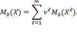
Given the additive form of equation (5.7), it is also possible to compute the contribution of each subgroup to overall poverty. Let us denote the contribution of subgroup ![]() to overall poverty by
to overall poverty by ![]() , which is formulated as
, which is formulated as
|
|
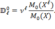
Note that the contribution of subgroup ![]() to overall poverty depends both on the level of poverty in subgroup
to overall poverty depends both on the level of poverty in subgroup![]() and on the population share of the subgroup. Whenever the contribution to poverty of a region or some other group greatly exceeds its population share, this suggests that there is a seriously unequal distribution of poverty in the country, with some regions or groups bearing a disproportionate share of poverty. Clearly, the sum of the contributions of all groups needs to be 100%.[13]
and on the population share of the subgroup. Whenever the contribution to poverty of a region or some other group greatly exceeds its population share, this suggests that there is a seriously unequal distribution of poverty in the country, with some regions or groups bearing a disproportionate share of poverty. Clearly, the sum of the contributions of all groups needs to be 100%.[13]
5.5.2.1 Subgroup Decompositions of the Adjusted Headcount Ratio ()
Let us consider the example of the hypothetical society presented in Box 5.1 and show how the contribution of subgroups to the overall Adjusted Headcount Ratio is computed. For this example, let us assume a certain weighting structure and a certain poverty cutoff to identify who among these four persons is poor. We assume that a 40% weight is attached to income, a 25% weight is attached to years of education, and 25% weight is attached to undernourishment and the remaining 10% weight is attached to the access to improved sanitation. Thus, the weight vector is ![]() . We identify a person as poor if the person is deprived in 40% or more of weighted indicators, that is,
. We identify a person as poor if the person is deprived in 40% or more of weighted indicators, that is, ![]() .
.
For subgroup decomposition, we divide the entire population in ![]() into two subgroups. Subgroup 1 consists of three persons, whereas Subgroup 2 consists of only one person as presented in Table 5.1. Note that the person in Subgroup 2 is deprived in all dimensions. We denote the achievement matrix of Subgroup 1 by
into two subgroups. Subgroup 1 consists of three persons, whereas Subgroup 2 consists of only one person as presented in Table 5.1. Note that the person in Subgroup 2 is deprived in all dimensions. We denote the achievement matrix of Subgroup 1 by ![]() and that of Subgroup 2 by
and that of Subgroup 2 by ![]() .
.
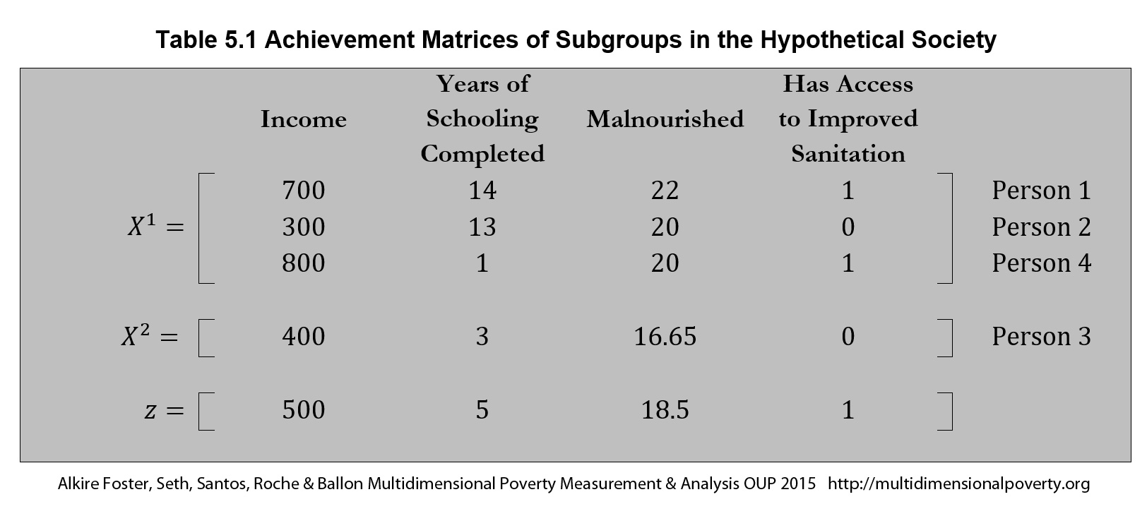
The deprivation matrices and deprivation scores of the two subgroups are presented in Table 5.2. Person 1 is not deprived in any dimension and so has a deprivation score of 0. Person 2 is deprived in two dimensions: standard of living and access to public services, and so the deprivation score is 0.375. Similarly, the deprivation score of Person 4 is 0.5 and Person 3’s is 1. Now, for ![]() , Person 2 and Person 4 are poor in Subgroup 1 and Person 3 is poor in Subgroup 2. In both subgroups, those who are deprived are identified as poor, and so there is no scope for censoring. The censored deprivation matrices for both groups are, in this particular case, the corresponding deprivation matrices.
, Person 2 and Person 4 are poor in Subgroup 1 and Person 3 is poor in Subgroup 2. In both subgroups, those who are deprived are identified as poor, and so there is no scope for censoring. The censored deprivation matrices for both groups are, in this particular case, the corresponding deprivation matrices.
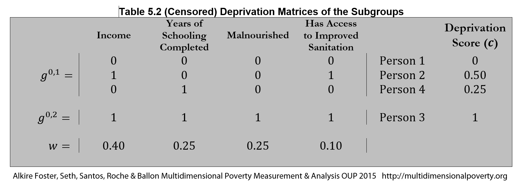
Thus, ![]() and
and ![]() . The overall Adjusted Headcount Ratio
. The overall Adjusted Headcount Ratio ![]() . It is straightforward to verify that the sum of the population-weighted Adjusted Headcount Ratios of subgroups is equal to the overall Adjusted Headcount Ratio. The population share of Subgroup 1 is
. It is straightforward to verify that the sum of the population-weighted Adjusted Headcount Ratios of subgroups is equal to the overall Adjusted Headcount Ratio. The population share of Subgroup 1 is ![]() and that of Subgroup 2 is
and that of Subgroup 2 is ![]() . Therefore,
. Therefore, ![]() .
.
Note that the Adjusted Headcount Ratio in Subgroup 2 is more than three times larger than the Adjusted Headcount Ratio of Subgroup 1. Does this mean that the contribution of Subgroup 2 is equally large? Not necessarily. It may not always be the case because of different population sizes across different subgroups. Recall that the contribution of a subgroup to overall poverty depends on the population share of that subgroup as well. For our example, the contribution of Subgroup 1 to the overall Adjusted Headcount Ratio is ![]() or 42.8%. The contribution of Subgroup
or 42.8%. The contribution of Subgroup ![]() to the overall headcount ratio is
to the overall headcount ratio is ![]() or 57.1%. It is worth noting that, in this case, the population Subgroup 2 does bear a disproportionate load of poverty since, despite being only 25% of the total population, it contributes nearly 60% of overall poverty. Because population shares affect interpretation, tables showing subgroup decompositions must include population shares for each subgroup, as well as poverty figures.
or 57.1%. It is worth noting that, in this case, the population Subgroup 2 does bear a disproportionate load of poverty since, despite being only 25% of the total population, it contributes nearly 60% of overall poverty. Because population shares affect interpretation, tables showing subgroup decompositions must include population shares for each subgroup, as well as poverty figures.
5.5.3 Dimensional Breakdown
As discussed in section 2.5, a multidimensional poverty measure that satisfies the dimensional breakdown property can be expressed as a weighted sum of the dimensional deprivations after identification. The ![]() satisfies the dimensional breakdown property and thus can also be expressed as a weighted sum of post-identification dimensional deprivation, which in the particular case of
satisfies the dimensional breakdown property and thus can also be expressed as a weighted sum of post-identification dimensional deprivation, which in the particular case of ![]() we refer to as the censored headcount ratio.
we refer to as the censored headcount ratio.
Why is this property useful? This property allows one to analyse the composition of multidimensional poverty. For example, Alkire and Foster (2011a), after decomposing overall poverty in the United States by ethnic group, break the poverty within those groups down by dimensions and examine how different ethnic groups have different dimensional deprivations, i.e. different poverty compositions.
The censored headcount ratio of a dimension is defined as the percentage of the population who are both multidimensionally poor and simultaneously deprived in that dimension. Formally, we denote the ![]() th column of the censored deprivation matrix
th column of the censored deprivation matrix ![]() as
as ![]() and the mean of the column for that chosen dimension
and the mean of the column for that chosen dimension ![]() as
as ![]() . We define
. We define ![]() as the censored headcount ratio of dimension
as the censored headcount ratio of dimension ![]() . What is the interpretation of
. What is the interpretation of ![]() ? The censored headcount ratio
? The censored headcount ratio ![]() is the proportion of the population that are identified as poor (
is the proportion of the population that are identified as poor (![]() ) and are deprived in dimension
) and are deprived in dimension ![]() .
.
The additive structure of the ![]() measure allows it to be expressed as a weighted sum of the censored headcount ratios, where the weight on dimension
measure allows it to be expressed as a weighted sum of the censored headcount ratios, where the weight on dimension ![]() is the relative weight assigned to that dimension. We have already seen in expression (5.3) that
is the relative weight assigned to that dimension. We have already seen in expression (5.3) that ![]() . This expression can be reformulated as
. This expression can be reformulated as
Analyses based on the censored headcount ratios can be complemented in an interesting way by considering the percentage contribution of each dimension to overall poverty. The censored headcount ratio shows the extent of deprivations among the poor but not the relative value of the dimensions. Two dimensions may have the same censored headcount ratios but very different contributions to overall poverty. This is because the contribution not only depends on the censored headcount ratio but also on the weight or value assigned to each dimension. Let us denote the contribution of dimension ![]() to the
to the ![]() by
by ![]() . Then, the contribution of dimension
. Then, the contribution of dimension ![]() for poverty cutoff
for poverty cutoff ![]() is given by
is given by
|
|
for each ![]() . Whenever the contribution to poverty of a certain indicator greatly exceeds its weight, there is a relatively high censored headcount in this indicator. The poor are more deprived in this indicator than in others. Clearly, the sum of the contributions of all indicators is 100%.[14] The censored headcount ratios and the percentage contributions have policy relevance for understanding the composition of poverty in different regions. Chapter 9 describes how they may be used to analyse intertemporal changes in multidimensional poverty and percentage contributions.
. Whenever the contribution to poverty of a certain indicator greatly exceeds its weight, there is a relatively high censored headcount in this indicator. The poor are more deprived in this indicator than in others. Clearly, the sum of the contributions of all indicators is 100%.[14] The censored headcount ratios and the percentage contributions have policy relevance for understanding the composition of poverty in different regions. Chapter 9 describes how they may be used to analyse intertemporal changes in multidimensional poverty and percentage contributions.
The uncensored (raw) headcount ratio of a dimension is defined as the proportion of the population that are deprived in that dimension. It aggregates deprivations pertaining to the poor (censored headcount) with deprivations among the non-poor. The uncensored headcount ratio of dimension ![]() is computed from the
is computed from the ![]() th column
th column ![]() of the (uncensored) deprivation matrix
of the (uncensored) deprivation matrix ![]() . We denote the mean of the column vector
. We denote the mean of the column vector ![]() by
by ![]() . Therefore,
. Therefore, ![]() is the uncensored (raw) headcount ratio of dimension
is the uncensored (raw) headcount ratio of dimension ![]() .
.
The censored headcount ratio may differ from the uncensored headcount ratio except when the identification criterion used is union. In this case, a person is identified as poor if the person is deprived in any dimension, so no deprivations are censored. Thus, the censored and uncensored headcount ratios are identical.
5.5.3.1 The Censored and Uncensored Headcount Ratios and Percentage Contributions
Using a hypothetical illustration, we now show how the uncensored headcount ratios and the censored headcount ratios are computed and then show how the contribution of each dimension to the Adjusted Headcount Ratio is calculated. Let us consider the same achievement matrix and weight vector as was in the previous subsection, which consists of four persons and four dimensions.
First, we show how to compute the uncensored headcount ratio. The achievement matrix ![]() and the deprivation cutoff vector
and the deprivation cutoff vector ![]() are used obtain the deprivation matrix
are used obtain the deprivation matrix ![]() , presented in Table 5.3. The uncensored headcount ratio of any dimension
, presented in Table 5.3. The uncensored headcount ratio of any dimension ![]() is
is ![]() . The uncensored headcount ratio of the standard of living dimension is
. The uncensored headcount ratio of the standard of living dimension is ![]() . In other words, 50% of the population is deprived in the standard of living dimension. Similarly, the uncensored headcount ratio of the knowledge dimension is 50%, of the nutritional status dimension is 25% and of the access to services dimension is 50%. The uncensored headcount ratios (summarized by vector
. In other words, 50% of the population is deprived in the standard of living dimension. Similarly, the uncensored headcount ratio of the knowledge dimension is 50%, of the nutritional status dimension is 25% and of the access to services dimension is 50%. The uncensored headcount ratios (summarized by vector ![]() ) are reported in the bottom-most row of the table.
) are reported in the bottom-most row of the table.

Next, we show how to compute the censored headcount ratio. We identify a person as poor if the person is deprived in 40% of weighted indicators, i.e. ![]() . Using the identification function we construct the censored deprivation matrix, presented in Table 5.4. Note that we censor the deprivations of Person 4 and replace them by 0 even when Person 4 is deprived in the education dimension. Why do we do this? We do so because the deprivation score of Person 4 is only 0.25, which is less than the poverty cutoff of
. Using the identification function we construct the censored deprivation matrix, presented in Table 5.4. Note that we censor the deprivations of Person 4 and replace them by 0 even when Person 4 is deprived in the education dimension. Why do we do this? We do so because the deprivation score of Person 4 is only 0.25, which is less than the poverty cutoff of ![]() . It can be easily verified that the
. It can be easily verified that the ![]() measure obtained from the censored deprivation matrix is 0.350.
measure obtained from the censored deprivation matrix is 0.350.
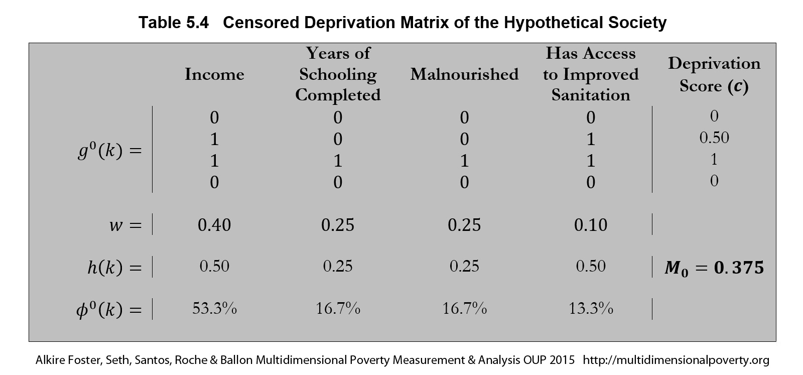
Let us finish this example by showing how to compute the contribution of a dimension to the Adjusted Headcount Ratio. We already know that the Adjusted Headcount Ratio is 0.350 and that the percentage contribution is ![]() . Let us consider the income dimension, which has a censored headcount ratio of 0.50 and the weight attached to it is 0.40. Then the contribution of the dimension to the Adjusted Headcount Ratio is
. Let us consider the income dimension, which has a censored headcount ratio of 0.50 and the weight attached to it is 0.40. Then the contribution of the dimension to the Adjusted Headcount Ratio is ![]() or 53.3%. Similarly, the contribution of the education dimension is
or 53.3%. Similarly, the contribution of the education dimension is ![]() or 16.7%. An interesting aspect to note is that the censored headcount ratio of the access to sanitation dimension is the same as that of the income dimension, but its contribution to the Adjusted Headcount Ratio is only 13.3%, which is lower than the contribution of the income dimension. The reason is that the weight attached to the standard of living dimension is twice the weight of these two dimensions.
or 16.7%. An interesting aspect to note is that the censored headcount ratio of the access to sanitation dimension is the same as that of the income dimension, but its contribution to the Adjusted Headcount Ratio is only 13.3%, which is lower than the contribution of the income dimension. The reason is that the weight attached to the standard of living dimension is twice the weight of these two dimensions.
5.6 A Case Study: The Global Multidimensional Poverty Index (MPI)
Now that we have learned how to compute the Adjusted Headcount Ratio and its partial indices, we provide an example showing one prominent implementation of the ![]() measure: the global Multidimensional Poverty Index (MPI). The global MPI was introduced by Alkire and Santos (2010) and has been reported annually in the Human Development Report since 2010.[15] The index consists of ten indicators grouped into three dimensions as outlined in Table 5.5.
measure: the global Multidimensional Poverty Index (MPI). The global MPI was introduced by Alkire and Santos (2010) and has been reported annually in the Human Development Report since 2010.[15] The index consists of ten indicators grouped into three dimensions as outlined in Table 5.5.

Note that the index uses nested weights. The weights are distributed such that each dimension reported in the first column receives an equal weight of 1/3 and the weight is equally divided among indicators within each dimension (note the distinction in terms here between indicator and dimension). Thus, each education and health indicator receives larger weights than the standard of living indicators. The weights for each indicator are reported in the third column. The deprivation cutoffs are outlined in the final column. Any person living in a household that fails to meet the deprivation cutoff is identified as deprived in that indicator. An abbreviation has been assigned to each indicator in the second column that will be useful for the presentations in next table.
Table 5.6 presents a hypothetical example of people living in four households, which will help explain how the MPI is constructed. The first two households live in urban areas and the third and the fourth households live in rural areas. In this illustration, the households are not of equal size. The household sizes are reported in the third column of the table. The deprivation matrix (![]() ) is presented in columns 4 through column 13. Following the standard notation, a 1 indicates that a household is deprived in the corresponding indicator and 0 indicates that the household is not deprived in that indicator. For example, the first household is only deprived in mortality (M) and cooking fuel (C), whereas the fourth household is deprived in five indicators: schooling (Sc), mortality (M), electricity (E), cooking fuel (C), and asset ownership (A).
) is presented in columns 4 through column 13. Following the standard notation, a 1 indicates that a household is deprived in the corresponding indicator and 0 indicates that the household is not deprived in that indicator. For example, the first household is only deprived in mortality (M) and cooking fuel (C), whereas the fourth household is deprived in five indicators: schooling (Sc), mortality (M), electricity (E), cooking fuel (C), and asset ownership (A).

Let us first show how the deprivation score (![]() ) of each person is computed. Note that in this example, all persons within a household are assigned the same deprivation score, which is the weighted sum of deprivations that the household faces. For example, the deprivation score of each person in the first household is
) of each person is computed. Note that in this example, all persons within a household are assigned the same deprivation score, which is the weighted sum of deprivations that the household faces. For example, the deprivation score of each person in the first household is
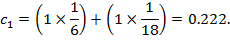
The deprivation scores are reported in column 14. The deprivation scores of the second, third, and fourth households are 0.72, 0.39, and 0.50, respectively. Thus, the second household has the largest deprivation score and the first household has the lowest deprivation score.
In the computation of the global MPI, a person is identified as poor if the person’s deprivation score is equal to 1/3 or higher. It is evident from column 14 that the first household’s deprivation score is less than 1/3, whereas the three other households’ deprivation scores are larger than 1/3. Thus, all persons in the first household are identified as non-poor, whereas all other persons in the last three households are identified as multidimensionally poor. Column 15 classifies the households as multidimensionally poor or not. The multidimensional headcount ratio or the incidence of poverty (![]() ) is (hint: use the household size)
) is (hint: use the household size)
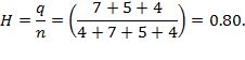
So 80% of the population are poor. Note that we have already discussed that the multidimensional headcount ratio (H) does not satisfy the dimensional monotonicity property, and so it does not change if any of the three poor households become deprived in an additional dimension. This limitation is overcome by the Adjusted Headcount Ratio (![]() ), which is called the MPI in this example. The censored deprivation scores are reported in column 16, where the deprivation score of the first household has been censored by replacing the score by 0. The MPI is the mean of the censored deprivation score vector and can be computed using expression (5.3) as (hint: use the household size)
), which is called the MPI in this example. The censored deprivation scores are reported in column 16, where the deprivation score of the first household has been censored by replacing the score by 0. The MPI is the mean of the censored deprivation score vector and can be computed using expression (5.3) as (hint: use the household size)
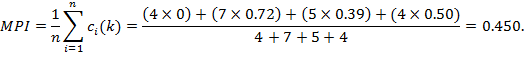
One may be also interested in knowing how poor the poor people are or the intensity of multidimensional poverty. The intensity of poverty can be computed as
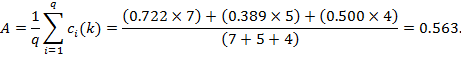
So, on average, poor people are deprived in 56.3% of the weighted indicators. It can be easily verified that the MPI is the product of the incidence of poverty and the intensity of poverty, i.e. ![]()
Let us now show how the subgroup decomposition property may be used to understand the subgroups’ multidimensional poverty and the contribution of the subgroup to the overall poverty. Using the same process as above, the ![]() ,
, ![]() , and
, and ![]() can be computed for each population subgroup. The MPI of the two urban households is 0.46, which can be obtained either by summing the censored deprivation scores weighted by the population share of each household or as a product of
can be computed for each population subgroup. The MPI of the two urban households is 0.46, which can be obtained either by summing the censored deprivation scores weighted by the population share of each household or as a product of ![]() and
and ![]() . The MPI of the two rural households is 0.44, whereas
. The MPI of the two rural households is 0.44, whereas ![]() and
and ![]() . Indeed, the incidence of poverty in the rural households is higher because all persons are identified as multidimensionally poor; whereas in the urban households this is not the case. However, when comparing the MPIs, we find the urban households have higher poverty because the intensity is higher. The urban households contribute 55% of the total population, and the rural ones contribute 45%. Thus, following the decomposition formula in equation (5.7), it can be verified that the overall MPI is
. Indeed, the incidence of poverty in the rural households is higher because all persons are identified as multidimensionally poor; whereas in the urban households this is not the case. However, when comparing the MPIs, we find the urban households have higher poverty because the intensity is higher. The urban households contribute 55% of the total population, and the rural ones contribute 45%. Thus, following the decomposition formula in equation (5.7), it can be verified that the overall MPI is ![]() . Again, using equation (5.8), it can be verified that the urban contribution to the overall MPI is 56%, whereas the rural contribution to the overall MPI is only 44%.
. Again, using equation (5.8), it can be verified that the urban contribution to the overall MPI is 56%, whereas the rural contribution to the overall MPI is only 44%.
Next, using the last rows of Table 5.6, we show how the dimensional breakdown property is used. We have seen in expression (5.9) that the overall ![]() can be expressed as a weighted average of censored headcount ratios. How are the censored headcount ratios in Table 5.6 computed? The censored headcount ratio for the years of education indicator is equal to (7+4)/20 = 55%. Similarly, the censored headcount ratio of the cooking fuel indicator is equal to (7+4+5)/20 = 80%. Note that the first household is not identified as poor and thus censored. This is why the censored headcount ratios are different from the uncensored headcount ratios reported in the row above. Looking at them, we can see that the poor in this society exhibit the highest deprivation levels in access to electricity and cooking fuel, followed (though with much lower headcount ratios) by sanitation, years of education, mortality, and assets. The percentage contributions of the indicators, which are computed using expression (5.10), are reported in the final column of the table. It is evident that neither electricity nor sanitation nor assets have the highest contribution to the overall MPI. Why? Because the weights assigned to these dimensions are lower than those assigned to schooling and mortality.
can be expressed as a weighted average of censored headcount ratios. How are the censored headcount ratios in Table 5.6 computed? The censored headcount ratio for the years of education indicator is equal to (7+4)/20 = 55%. Similarly, the censored headcount ratio of the cooking fuel indicator is equal to (7+4+5)/20 = 80%. Note that the first household is not identified as poor and thus censored. This is why the censored headcount ratios are different from the uncensored headcount ratios reported in the row above. Looking at them, we can see that the poor in this society exhibit the highest deprivation levels in access to electricity and cooking fuel, followed (though with much lower headcount ratios) by sanitation, years of education, mortality, and assets. The percentage contributions of the indicators, which are computed using expression (5.10), are reported in the final column of the table. It is evident that neither electricity nor sanitation nor assets have the highest contribution to the overall MPI. Why? Because the weights assigned to these dimensions are lower than those assigned to schooling and mortality.
We now provide the following example to show how the censored headcount ratio and the percentage contribution of dimensions are used in practice. Borrowing from Alkire, Roche, and Seth (2011), the example provides information on two subnational regions for a cross-country implementation of the MPI. These two regions have roughly the same ![]() levels reported in the final row of Table 5.7. Breaking
levels reported in the final row of Table 5.7. Breaking ![]() down by dimension reveals how the underlying structure of deprivations differs across the two countries for the ten indicators.[19] In Ziguinchor (a region in Senegal), mortality deprivations contribute the most to multidimensional poverty, whereas in Barisal (a division in Bangladesh), the relative contribution of nutritional deprivations is much larger than, say, deprivations in school attendance. Although the overall poverty levels as measured by
down by dimension reveals how the underlying structure of deprivations differs across the two countries for the ten indicators.[19] In Ziguinchor (a region in Senegal), mortality deprivations contribute the most to multidimensional poverty, whereas in Barisal (a division in Bangladesh), the relative contribution of nutritional deprivations is much larger than, say, deprivations in school attendance. Although the overall poverty levels as measured by ![]() are very similar, dimensional breakdown reveals a very different underlying structure of poverty, which in turn could suggest different policy responses.
are very similar, dimensional breakdown reveals a very different underlying structure of poverty, which in turn could suggest different policy responses.
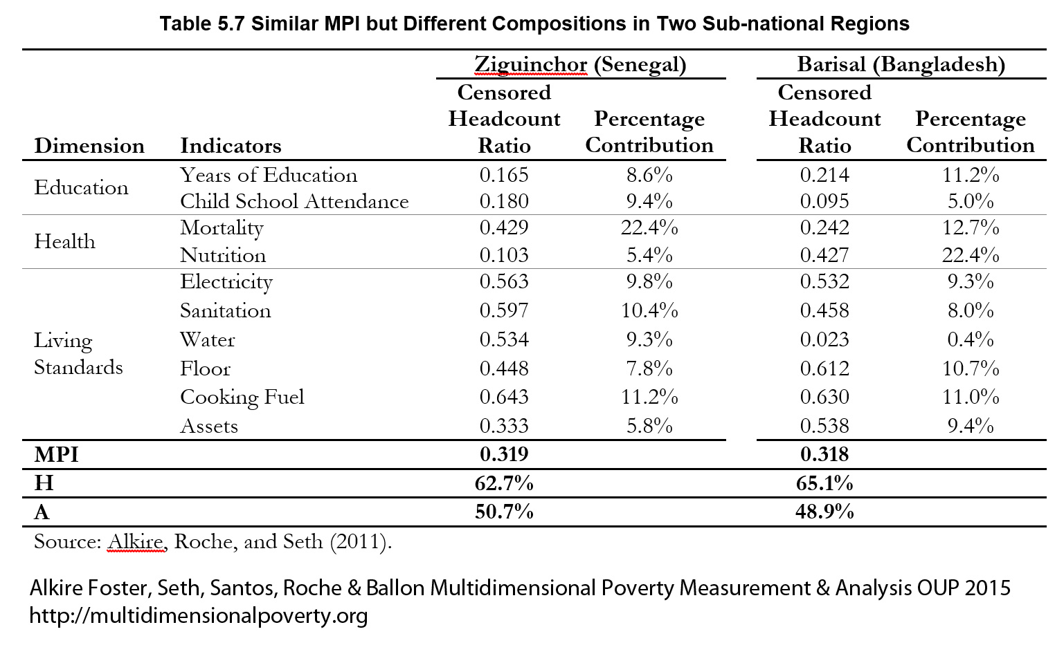
5.7 AF Class Measures Used with Cardinal Variables
In this chapter our discussion has focused on the Adjusted Headcount Ratio as many poverty indicators in practice are of ordinal scale. However, if all indicators are cardinal, we can go beyond the Adjusted Headcount Ratio to measures that additionally reflect the depth of deprivations poor people experience below the deprivation cutoff in each dimension. The identification step proceeds in exactly the same way as with ![]() . The difference is in the aggregation step. This section introduces the normalized gap matrix, which is used for the aggregation step for all the
. The difference is in the aggregation step. This section introduces the normalized gap matrix, which is used for the aggregation step for all the ![]() class of measures with
class of measures with ![]() . The section also presents the two most common members of the
. The section also presents the two most common members of the ![]() class with
class with ![]() :
: ![]() and
and ![]() .
.
5.7.1 The Normalized Gap Matrix
The basic matrix for measures drawing upon cardinal data is the normalized gap matrix, which, like the deprivation matrix, is constructed from the achievement matrix and the vector of deprivation cutoffs. The entries in the normalized gap matrix are the shortfall or gap in deprived people’s achievements, expressed as a proportion of the respective dimensional deprivation cutoff.
In the normalized gap matrix ![]() the typical element is defined by
the typical element is defined by ![]() . In other words, the normalized gap matrix replaces each deprived entry in
. In other words, the normalized gap matrix replaces each deprived entry in ![]() with the respective normalized gap and replaces each entry that is not below its deprivation cutoff with 0. The normalized gap matrix provides a snapshot of the depth of deprivation of each person in each dimension. The squared gap matrix
with the respective normalized gap and replaces each entry that is not below its deprivation cutoff with 0. The normalized gap matrix provides a snapshot of the depth of deprivation of each person in each dimension. The squared gap matrix ![]() replaces each deprived entry in
replaces each deprived entry in ![]() with the square of the normalized gap and replaces each entry that is not below its deprivation cutoff with 0. Thus the typical element of the squared gap matrix is
with the square of the normalized gap and replaces each entry that is not below its deprivation cutoff with 0. Thus the typical element of the squared gap matrix is ![]() . Squaring the normalized gaps puts relatively more emphasis on larger deprivations. Generalizing the above, we may define the normalized gap matrix of order
. Squaring the normalized gaps puts relatively more emphasis on larger deprivations. Generalizing the above, we may define the normalized gap matrix of order ![]() by raising the normalized gaps to the power
by raising the normalized gaps to the power ![]() and denote this by
and denote this by ![]() , whose typical element is
, whose typical element is ![]() . Clearly, if the normalized gap matrix is raised to the power 0, we would return to the deprivation matrix
. Clearly, if the normalized gap matrix is raised to the power 0, we would return to the deprivation matrix ![]() , in which all entries take the value of 0 or 1. Similarly, if the normalized gap matrix is raised to the power one and two, we obtain
, in which all entries take the value of 0 or 1. Similarly, if the normalized gap matrix is raised to the power one and two, we obtain ![]() and
and ![]() , respectively.
, respectively.
From the normalized gap matrices, we apply the same identification function ![]() to obtain the censored normalized gap matrix of order
to obtain the censored normalized gap matrix of order ![]() as
as ![]() such that
such that ![]() . Recall that the identification function
. Recall that the identification function ![]() is based on the vector of weighted deprivation counts
is based on the vector of weighted deprivation counts ![]() (generated, as before, from the
(generated, as before, from the ![]() matrix and the vector of weights) and the poverty cutoff
matrix and the vector of weights) and the poverty cutoff ![]() . The identification function replaces all deprived entries of the non-poor with 0 and leaves the deprived entries of the poor unchanged. We define
. The identification function replaces all deprived entries of the non-poor with 0 and leaves the deprived entries of the poor unchanged. We define ![]() as the censored normalized gap matrix and
as the censored normalized gap matrix and ![]() as the censored squared gap matrix.
as the censored squared gap matrix.
5.7.2 The Adjusted Poverty Gap, Adjusted FGT, and Ma Measures
The Adjusted Poverty Gap measure ![]() can be defined as
can be defined as
|
|
(5.11) |
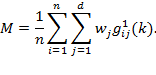
In other words, the Adjusted Poverty Gap is the sum of the weighted normalized gaps of the poor or ![]() divided by the population (
divided by the population (![]() ). Another way of viewing
). Another way of viewing ![]() is in terms of partial indices:
is in terms of partial indices: ![]() is the product of
is the product of ![]() (incidence) and
(incidence) and ![]() (intensity) (which in turn is
(intensity) (which in turn is ![]() ) and the average deprivation gap among the poor
) and the average deprivation gap among the poor ![]() . That is,
. That is,
|
|
(5.12) |
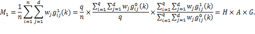
In words, ![]() is the average value of the normalized gap among all instances in which any poor person is deprived (and hence where the censored normalized gap is positive). Thus,
is the average value of the normalized gap among all instances in which any poor person is deprived (and hence where the censored normalized gap is positive). Thus, ![]() provides information on the average depth of deprivations across all poor and deprived states.
provides information on the average depth of deprivations across all poor and deprived states.
As in the case of ![]() , the partial indices greatly aid in comparing multidimensional poverty across time and space. Suppose for example that
, the partial indices greatly aid in comparing multidimensional poverty across time and space. Suppose for example that ![]() is higher in one region than in another. It could be useful to examine the extent to which the difference is due to a higher
is higher in one region than in another. It could be useful to examine the extent to which the difference is due to a higher ![]() ,or to higher values of
,or to higher values of ![]() or
or ![]() It is also possible to examine the average gaps for each dimension to identify in which dimension normalized gaps tend to be higher.
It is also possible to examine the average gaps for each dimension to identify in which dimension normalized gaps tend to be higher.
Under methodology (![]() ), if the deprivation of a poor person deepens in any dimension, then the respective
), if the deprivation of a poor person deepens in any dimension, then the respective ![]() will rise and hence so will
will rise and hence so will ![]() . Consequently, (
. Consequently, (![]() ) satisfies the property of monotonicity.
) satisfies the property of monotonicity.
To incorporate sensitivity to one form of inequality among the poor, which satisfies the transfer property defined in section 2.5, we turn to the censored matrix ![]() of squared normalized shortfalls. The Adjusted Squared Gap measure or Adjusted FGT Measure
of squared normalized shortfalls. The Adjusted Squared Gap measure or Adjusted FGT Measure ![]() can be defined as
can be defined as
|
|
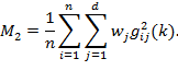
The adjusted squared gap is the sum of the weighted normalized squared gaps of the poor, or ![]() divided by the population (
divided by the population (![]() ).
). ![]() can also be expressed in terms of partial indices as the product of
can also be expressed in terms of partial indices as the product of ![]() (incidence) and
(incidence) and ![]() (intensity) and the average severity index
(intensity) and the average severity index ![]() . That is
. That is
|
|
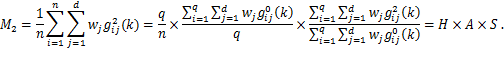
The average severity index ![]() denotes the average severity among all instances where a poor person is deprived (and hence where the censored squared gap is positive). By summarizing the square of the normalized gaps,
denotes the average severity among all instances where a poor person is deprived (and hence where the censored squared gap is positive). By summarizing the square of the normalized gaps, ![]() places relatively greater emphasis on the larger gaps. Therefore, under
places relatively greater emphasis on the larger gaps. Therefore, under ![]() , a given-sized increase in a deprivation of a poor person will have a greater impact the larger the initial level of deprivation. Consequently, the methodology satisfies the weak transfer property and is sensitive to the inequality with which deprivations are distributed among the poor.
, a given-sized increase in a deprivation of a poor person will have a greater impact the larger the initial level of deprivation. Consequently, the methodology satisfies the weak transfer property and is sensitive to the inequality with which deprivations are distributed among the poor.
We generalize ![]() ,
, ![]() , and
, and ![]() to the class
to the class ![]() of multidimensional poverty measures associated with the unidimensional FGT class. The adjusted FGT class of multidimensional poverty measures can be defined as
of multidimensional poverty measures associated with the unidimensional FGT class. The adjusted FGT class of multidimensional poverty measures can be defined as
|
|
(5.15) |
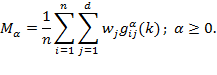
In other words, ![]() is the sum of the
is the sum of the![]() powers of the normalized gaps of the poor, or
powers of the normalized gaps of the poor, or ![]() divided by the population (
divided by the population (![]() ). In the notation (Method IV in Box 5.7) used in Alkire and Foster (2011a), the
). In the notation (Method IV in Box 5.7) used in Alkire and Foster (2011a), the ![]() ,
, ![]() and
and ![]() indices are each the means of their respective matrices.
indices are each the means of their respective matrices.
The general methodology employing the dual-cutoff function ![]() and an associated FGT measure
and an associated FGT measure ![]() is denoted by
is denoted by![]() It is important to define the AF methodology fully, both the dual-cutoff identification strategy and the poverty measures, because it is this combined methodology which assures that the resulting measures satisfy the principles here specified.
It is important to define the AF methodology fully, both the dual-cutoff identification strategy and the poverty measures, because it is this combined methodology which assures that the resulting measures satisfy the principles here specified.
As stated in section 3.6.1 and as a way to wrap up this chapter, it is worth recalling that all measures in the AF family satisfy symmetry, replication invariance, scale invariance, poverty focus, deprivation focus, dimensional monotonicity, population subgroup decomposability, and dimensional breakdown. For ![]() , the measure satisfies the ordinality property, making it suitable for implementation when at least some of the indicators used are of ordinal scale. For
, the measure satisfies the ordinality property, making it suitable for implementation when at least some of the indicators used are of ordinal scale. For ![]() , the measures require all indicators to be cardinal. When
, the measures require all indicators to be cardinal. When![]() , the measures satisfy strong monotonicity. When
, the measures satisfy strong monotonicity. When![]() , the measures satisfy transfer and weak deprivation rearrangement. When the union criterion is used for identification and
, the measures satisfy transfer and weak deprivation rearrangement. When the union criterion is used for identification and ![]() , the measures satisfy continuity.
, the measures satisfy continuity.
Box 5.6 α An Alternative Presentation of ![]() Measures Using Non-normalized Weights
Measures Using Non-normalized Weights
In this chapter we have stated the formulas in terms of normalized weights (Method I in Box 5.7), but they can also be expressed using non-normalized weights such that ![]() for all
for all ![]() and
and ![]() , so that they add to the total number of dimensions (Method IV in Box 5.7). In order to do so, we introduce the weighted normalized gap matrices. Like the weighted deprivation matrix
, so that they add to the total number of dimensions (Method IV in Box 5.7). In order to do so, we introduce the weighted normalized gap matrices. Like the weighted deprivation matrix ![]() that we defined earlier in Box 5., we may also define the weighted normalized gap matrix of order
that we defined earlier in Box 5., we may also define the weighted normalized gap matrix of order ![]() as
as ![]() such that
such that ![]() . In other words, in weighted normalized gap matrices, each deprived entry in
. In other words, in weighted normalized gap matrices, each deprived entry in ![]() is replaced with its respective normalized gap of order
is replaced with its respective normalized gap of order ![]() multiplied by its relative weight and each entry that is not below its deprivation cutoff is replaced with 0. For
multiplied by its relative weight and each entry that is not below its deprivation cutoff is replaced with 0. For ![]() ,
, ![]() is the weighted normalized gap matrix with the typical element being
is the weighted normalized gap matrix with the typical element being ![]() . Similarly, for
. Similarly, for ![]() ,
, ![]() is the weighted squared gap matrix with
is the weighted squared gap matrix with ![]() .
.
The censored weighted normalized gap matrix of order ![]() can be obtained as
can be obtained as ![]() such that
such that ![]() . Thus,
. Thus, ![]() is the censored weighted normalized gap matrix and
is the censored weighted normalized gap matrix and ![]() is the censored weighted normalized squared gap matrix. As with any censored matrix, these matrices are obtained by multiplying the (weighted) deprivation matrix by the identification function
is the censored weighted normalized squared gap matrix. As with any censored matrix, these matrices are obtained by multiplying the (weighted) deprivation matrix by the identification function ![]() .
.
The adjusted FGT class of multidimensional poverty measures can be defined as
|
|
In this case, ![]() is the weighted sum of the α powers of the normalized gaps of the poor, or
is the weighted sum of the α powers of the normalized gaps of the poor, or ![]() divided by the highest possible value for this sum, or
divided by the highest possible value for this sum, or ![]() .
.
Based on expression (5.16), the Adjusted Poverty Gap measure ![]() is the mean of the censored weighted normalized gap matrix and can be defined as
is the mean of the censored weighted normalized gap matrix and can be defined as
|
|
(5.17) |
Thus, the Adjusted Poverty Gap is the sum of the weighted normalized gaps of the poor, or ![]() divided by the highest possible sum of normalized gaps, or
divided by the highest possible sum of normalized gaps, or ![]() .
.
Similarly, the Adjusted Squared Gap or the Adjusted FGT Measure is given by
|
|
(5.18) |
Thus, ![]() is the sum of the squared normalized gaps of the poor, or
is the sum of the squared normalized gaps of the poor, or ![]() , divided by the highest possible sum of the squared normalized gaps, or
, divided by the highest possible sum of the squared normalized gaps, or ![]() .
.
5.8 Some Implementations of the AF Methodology
As mentioned in Chapter 1, since its development, the Alkire-Foster approach to multidimensional poverty has generated some practical interest. These include a global Multidimensional Poverty Index (MPI) estimated over 100 developing countries[20] as well as official national multidimensional poverty measures in Mexico, Colombia, Bhutan, and the Philippines with many other regional, national and subnational measures in progress.[21] Adaptations of the methodology include the Gross National Happiness Index of the Royal Government of Bhutan (Ura et al. 2012) and the Women’s Empowerment in Agriculture Index (Alkire, Meinzen-Dick et al. 2013). Several academic studies have implemented the AF approach for different poverty measurement purposes and in different parts of the world. These are summarized in Table 5.8.
Table 5.8. Summary of Research Studies That Have Implemented the AF Methodology
|
Authors |
Year |
Paper Title |
Implements AF |
Region of the world for which it was |
|
Alkire Apablaza and Jung |
2014 |
Multidimensional Poverty Measurement for EU-SILC countries |
Constructs trial measures using EU-SILC data 2006–2012 and analyses by country, gender, age, and dimensional composition |
Europe |
|
Alkire and Seth |
2013a |
Identifying BPL Households: A Comparison of Methods |
Compares a simple targeting-based method to some of the proposed mthods for targeting the poor for the BPL programme in India. |
India, South Asia |
|
Alkire and Seth |
2013b |
Multidimensional Poverty Reduction in India between 1999 and 2006: Where and How? |
Monitors and studies multidimensional poverty reduction in India |
India, South Asia |
|
Alkire and Seth |
2013c |
Selecting a Targeting Method to Identify BPL Households in India |
Propose a counting-based targeting methodology for the BPL programme in India |
India, South Asia |
|
Arndt et al |
2012 |
Ordinal Welfare Comparisons with Multiple Discrete Indicators: A First-Order Dominance Approach and Application to Child Poverty |
Performs child poverty comparison over time and between regions |
Vietnam, Mozambique |
|
Azevedo and Robles |
2013 |
Multidimensional Targeting: Identifying Beneficiaries of Conditional Cash Transfer Programmes |
Implements the AF methodology to propose a targeting method |
Latin America |
|
Batana |
2013 |
Multidimensional Measurement of Poverty Among Women in Sub-Saharan Africa |
Measure multidimensional poverty among women in fourteen sub-Saharan African countries |
Sub-Saharan Africa |
|
Battiston et al |
2013 |
Income and Beyond: Multidimensional Poverty in Six Latin American Countries |
Measure multidimensional poverty in six Latin American countries and track its reduction between 1992–2006 |
Latin America |
|
Beja and Yap |
2013 |
Counting Happiness from the Individual Level to the Group Level |
Uses the counting measure to assess group-level happieness |
Philippines |
|
Castro, Baca, Ocampo |
2012 |
(Re)counting the Poor in Peru: A Multidimensional Approach |
Uses the AF methodology to compare headcount ratios of monetary povery and multidimensional poverty between 2004 and 2008 in regions of Peru. |
Peru, Latin America |
|
Foster, Horowitz and Méndez |
2012 |
An Axiomatic Approach to the Measurement of Corruption: Theory and Applications |
Develops a measure of corruption |
No regional application |
|
Gradín |
2013 |
Race, Poverty and Deprivation in South Africa |
Measures poverty and material deprivation and the racial gap among South Africans after apartheid |
South Africa |
|
Mitra |
2013 |
Towards a Multidimensional Measure of Governance |
Develops a governance index for sub-Saharan African countries |
Sub-Saharan Africa |
|
Mitra, Posarac and Vick |
2013 |
Disability and Poverty in Developing Countries: A Multidimensional Study |
Obtains the economic profile of persons (aged 18–65) with disabilities. Multidimensional poverty analysis is performed for persons with and without disability |
Burkina Faso, Ghana, Kenya, Malawi, Mauritius, Zambia, and Zimbabwe; Bangladesh, Lao PDR, Pakistan, and the Philippines; Brazil, Dominican Republic, Mexico, and Paraguay |
|
Mitra, Jones et al. |
2013 |
Implementing a Multidimensional Poverty Measure Using Mixed Methods and a Participatory Framework |
Measures multidimensional poverty among people with psychiatric diagnoses. |
USA |
|
Nicholas and Ray |
2011 |
Duration and Persistence in Multidimensional Deprivation: Methodology and Australian Application |
Constructs dynamic deprivation measures and assesses the duration of deprivation across multiple dimensions |
Australia |
|
Notten and Roelen |
2012 |
A New Tool for Monitoring (Child) Poverty: Measures of Cumulative Deprivation |
Measures material deprivation, cumulative deprivation, child poverty. |
UK, Germany, France, the Netherlands |
|
Nussbaumer et al. |
2012 |
Measuring Energy Poverty: Focusing on What Matters |
Derives the Multidimensional Energy Poverty Index (MEPI) |
Angola, Benin, Burkina Faso, Cameroon, Congo Brazzaville, Congo Democratic Republic, Egypt, Ethiopia, Ghana, Guinea, Kenya, Lesotho, Liberia, Madagascar, Malawi, Mali, Morocco, Mozambique, Namibia, Niger, Nigeria, Rwanda, Senegal, Sierra Leone, Swaziland, Tanzania, Uganda, Zambia, Zimbabwe |
|
Peichl and Pestel |
2013a |
Multidimensional Affluence: Theory and Applications to Germany and the US |
Constructs an index of affluence instead of poverty to study affluence in Germany and the US |
Germany, USA |
|
Peichl and Pestel |
2013b |
Multidimensional Well-Being at the Top: Evidence for Germany |
Constructs an index of well-being to study well-being in Germany |
Germany |
|
Roche |
2013 |
Monitoring Progress in Child Poverty Reduction: Methodological Insights and Illustration to the Case Study of Bangladesh |
Measures multidimensional poverty among children in Bangladesh and analyze the patterns of poverty reduction. |
Bangladesh, South Asia |
|
Saini |
2013 |
Has Poverty Decreased in Cameroon between 2001 and 2007? An Analysis Based on Multidimensional Poverty Measures |
Analyses changes in multidimensional poverty in Cameroon between 2001 and 2007. |
Cameroon, sub-Saharan Africa |
|
Santos |
2013 |
Tracking Poverty Reduction in Bhutan: Income Deprivation Alongside Deprivation in Other Sources of Happiness |
Measure multidimensional poverty in Bhutan and track its trend between 2003 and 2007 |
Bhutan, South Asia |
|
Siegel and Waidler |
2012 |
Migration and Multi-Dimensional Poverty in Moldovan Communities |
Examines multidimnesional poverty in 180 Moldovian communities in 2011 |
Moldova, Eastern Europe |
|
Trani and Cannings |
2013 |
Child Poverty in an Emergency and Conflict Context: A Multidimensional Profile and an Identification of the Poorest Children in Western Darfur |
Measure child poverty |
Darfur, Sudan |
|
Tonmoy |
2014 |
An Exercise to Evaluate an Anti-Poverty Program with Multiple Outcomes Using Program Evaluation |
Evaluates a programme using multidimensional poverty measures with difference-in-difference matching estimators |
Bangladesh |
|
Trani et al |
2013 |
The Multidimensionality of Child Poverty: Evidence from Afghanistan |
Measures poverty among children in Afghanistan |
Afghanistan |
|
Yu |
2013 |
Multidimensional Poverty in China: Findings based on the CHNS |
Measures multidimensional poverty in China and track its progress between 2000 and 2009. |
China |
|
Wagle |
2014 |
The Counting-Based Measurement of Multidimensional Poverty: The Focus on Economic Resources, Inner Capabilities, and Relational Resources in the United States |
Comparing a two-step process of the dimensional approach to AF method |
USA |
Other papers do not directly implement the AF methodology but engage with it in various ways. These include Ferreira (2011), Ravallion (2011b) and others in the Journal of Economic Inequality, vol. 9 (2011), Ferreira and Lugo (2013), Ravallion (2012), Foster et al. (2010), Betti et al. (2012), Cardenas and Carpenter (2013), Larochelle (2014), Berenger et al. (2013), Siminski and Yerokhin (2012), and Smith (2012).
Chapter 6 which follows explains the normative decisions required to apply the AF framework of multidimensional poverty measurement empirically. It identifies the different decisions required, delineate their normative content and key considerations, and presents alternative courses of action.
Glossary
Note: This figure uses the normalized notation in which weights ![]() sum to 1 and
sum to 1 and ![]() , with the deprivation matrix.
, with the deprivation matrix.
|
Adjusted Headcount Ratio |
|
Alkire–Foster methodology |
|
Censored headcount ratios |
|
Censoring |
|
Decomposition |
|
Deprivation cutoffs ( |
|
Deprived |
|
Functionings |
|
Incidence ( |
|
Intensity ( |
|
Percentage contribution of each indicator |
|
Poor |
|
Poverty cutoff ( |
|
Uncensored or raw headcount ratios |
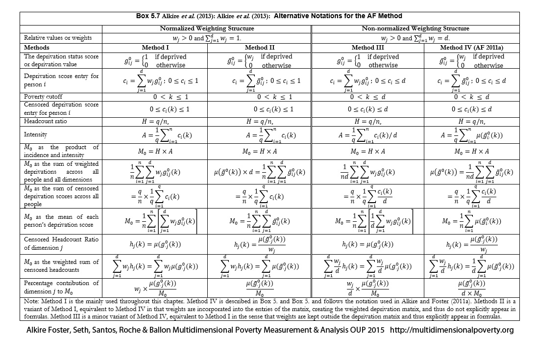
Bibliography
Alkire et al. (2013): Alkire, S., Meinzen-Dick, R., Peterman, A., Quisumbing, A. R., Seymour, G., and Vaz, A. (2013). ‘The Women’s Empowerment in Agriculture Index’. World Development, 53: 71–91.
Alkire et al. 2014a: Alkire, S., Conconi, A., and Seth, S. (2014). ‘Multidimensional Poverty Index 2014: Brief Methodological Note and Results’. OPHI MPI Methodological Note: MPI 2014.
Alkire, S. and Foster, J. (2007). ‘Counting and Multidimensional Poverty Measurement’. OPHI Working Paper 7, Oxford University.
Alkire, S. and Foster, J. (2011a). ‘Counting and Multidimensional Poverty Measurement’. Journal of Public Economics, 95(7–8): 476–487.
Alkire, S. and Santos, M. E. (2010). ‘Acute Multidimensional Poverty: A New Index for Developing Countries’. OPHI Working Paper 38, Oxford University; also published as Human Development Research Paper 2010/11.
Alkire, S. and Santos, M. E. (2013). ‘A Multidimensional Approach: Poverty Measurement and Beyond’. Social Indicators Research, 112(2): 239–257.
Alkire, S. and Santos, M. E. (2014). ‘Measuring Acute Poverty in the Developing World: Robustness and Scope of the Multidimensional Poverty Index’. World Development, 59: 251–274.
Alkire, S. and Seth, S. (2013a). ‘Identifying BPL Households’. Economic & Political Weekly, 48(2): 49–67.
Alkire, S. and Seth, S. (2013b). ‘Multidimensional Poverty Reduction in India between 1999 and 2006: Where and How?’ OPHI Working Paper 60, Oxford University.
Alkire, S. and Seth, S. (2013c). ‘Selecting a Targeting Method to Identify BPL Households in India’. Social Indicators Research 112 (2): 417–446.
Alkire, S., Apablaza, M., and Jung, E. (2014). ‘Multidimensional Poverty Measurement for EU-SILC countries’. OPHI Research in Progress 36c.
Alkire, S., Conconi, A., and Roche, J. M. (2013). ‘Multidimensional Poverty Index 2013: Brief Methodological Note and Results’. OPHI MPI Methodological Note: MPI 2013.
Alkire, S., Roche, J. M., and Seth S. (2011). ‘Sub-National Disparities and Inter-Temporal Evolution of Multidimensional Poverty across Developing Countries’. OPHI Research in Progress 32a, Oxford University.
Alkire, S., Roche, J. M., Santos, M. E., and Seth, S. (2011). ‘Multidimensional Poverty Index 2011: Brief Methodological Note’. OPHI Briefing 07.
Anand, S. and Sen, A. (1997). ‘Concepts of Human Development and Poverty: A Multidimensional Perspective’, in Human Development Papers 1997: Poverty and Human Development. UNDP, 1–20.
Arndt et al.: Arndt, C., Distante, R., Hussain, M. A., et al. (2012). ‘Ordinal Welfare Comparisons with Multiple Discrete Indicators: A First Order Dominance Approach and Application to Child Poverty’. World Development, 40(11): 2290–2301.
Atkinson, A. B. (2003). ‘Multidimensional Deprivation: Contrasting Social Welfare and Counting Approaches’. Journal of Economic Inequality, 1(1): 51–65.
Azevedo, V. and Robles, M. (2013). ‘Multidimensional Targeting: Identifying Beneficiaries of Conditional Cash Transfer Programs’. Social Indicators Research, 112(2): 447–475.
Batana, Y. M. (2013). ‘Multidimensional Measurement of Poverty Among Women in Sub-Saharan Africa’. Social Indicators Research, 112(2): 337–362.
Battiston et al. (2013): Battiston, D., Cruces, G., Lopez-Calva, L. F., Lugo, M. A., and Santos, M. E. (2013). ‘Income and Beyond: Multidimensional Poverty in Six Latin American Countries’. Social Indicators Research, 112(2): 291–314.
Beja, E. L., Jr. and Yap D. B. (2013). ‘Counting Happiness from the Individual Level to the Group Level’. Social Indicators Research, 114(2): 621–637.
Berenger et al. (2013): Berenger, V., Deutsch, J., and Silber, J. (2013). ‘Durable Goods, Access to Services and the Derivation of an Asset Index: Comparing Two Methodologies and Three Countries’. Economics Modeling, 35: 881–891.
Betti et al. (2012): Betti, G., Gagliardi, F., Lemmi, A., Verma, V.. (2012). ‘Subnational Indicators of Poverty and Deprivation in Europe: Methodology and Applications’. Cambridge Journal of Regions Economy and Society, 5(1): 129–147.
Bourguignon, F., and Chakravarty, S. R. (2003). ‘The Measurement of Multidimensional Poverty’. Journal of Economic Inequality, 1(1): 25–49.
Cardenas, J. C. and Carpenter, J. (2013). ‘Risk Attitudes and Economic Well-Being in Latin America’. Journal of Development Economics, 103(C): 52-61.
Castro et al. (2012): Castro, J. F., Baca, J., and Ocampo, J. P. (2012). ‘(Re)Counting the Poor in Peru: A Multidimensional Approach’. Latin American Journal of Economics-formerly Cuadernos de Economía, 49(1): 37-65, Instituto de Economía. Pontificia Universidad Católica de Chile.
Chakravarty et al. (1998): Chakravarty, S. R., Mukherjee, D., and Ranade, R. R. (1998). ‘On the Family of Subgroup and Factor Decomposability Measures of Multidimensional Poverty’, in D. J. Slottje (ed.), Research on Economic Inequality 8. JAI Press, 175–194.
DHS Bangladesh (2007): National Institute of Population Research and Training (NIPORT), Mitra and Associates, and Macro International. (2009). Bangladesh Demographic and Health Survey 2007. Dhaka, Bangladesh and Calverton, Maryland, U.S.A.
DHS Senegal (2005): Ndiaye, Salif, et Mohamed Ayad. (2006). Enquête Démographique et de Santé au Sénégal 2005. Calverton, Maryland, U.S.A., Centre de Recherche pour le Développement Humain [Sénégal] et ORC Macro.
Ferreira, F. H. G. (2011). ‘Poverty Is Multidimensional. But What Are We Going To Do About It?’ Journal of Economic Inequality, 9(3): 493–495.
Ferreira, F. H. G. and Lugo, M. A. (2013). ‘Multidimensional Poverty Analysis: Looking for a Middle Ground’. World Bank Research Observer, 28(2): 220–235.
Foster et al. (2010): Foster, J., Greer, J., and Thorbecke, E. (2010). ‘The Foster–Greer–Thorbecke (FGT) Poverty Measures: 25 Years Later’. Journal of Economic Inequality, 8(4): 491–524.
Foster et al. (2012): Foster, J. E., Horowitz A. W., and Méndez, F. (2012). ‘An Axiomatic Approach to the Measurement of Corruption: Theory and Applications’. World Bank Economic Review, 26(2): 217–235.
Foster J., Greer, J., and Thorbecke, E. (1984). ‘A Class of Decomposable Poverty Measures’. Econometrica, 52(3): 761–766.
Gradín, C. (2013). ‘Race, Poverty and Deprivation in South Africa’. Journal of African Economies, 22(2): 187–238.
Larochelle et al. (2014): Larochelle, C, Alwang, J., and Taruvinga, N. (2014). ‘Inter-temporal Changes in Well-being During Conditions of Hyperinflation: Evidence from Zimbabwe’. Journal of African Economics, 23(2): 225–256.
Mitra, S. (2013). ‘Towards a Multidimensional Measure of Governance’ Social Indicators Research. 112(2): 477–496
Mitra et al. (2013): Mitra, S., Jones, K., Vick, B., et al. (2013). ‘Implementing a Multidimensional Poverty Measure Using Mixed Methods and a Participatory Framework’. Social Indicators Research, 110(3): 1061–1081.
Mitra, S, Posarac, A., and Vick, B. (2013). ‘Disability and Poverty in Developing Countries: A Multidimensional Study’. World Development, 41: 1–18.
Nicholas, A. and Ray, R. (2012). ‘Duration and Persistence in Multidimensional Deprivation: Methodology and Australian Application’. Economic Record 88(280): 106–126.
Notten, G. and Roelen, K. (2012). ‘A New Tool for Monitoring (Child) Poverty: Measures of Cumulative Deprivation’. Child Indicators Research, 5(2): 335–355.
Nussbaumer et al. (2012): Nussbaumer, P., Bazilian, M., and Modi, V. (2012). ‘Measuring Energy Poverty: Focusing on what Matters’. Renewable & Sustainable Energy Reviews, 16(1): 231–243.
Pattanaik, P. K. and Xu, Y. (1990). ‘On Ranking Opportunity Sets in Terms of Freedom of Choice’. Recherches Economiques de Louvain. 56, 383-390.
Peichl, A. and Pestel, N. (2013a). ‘Multidimensional Affluence: Theory and Applications to Germany and the US.’ Applied Economics, 45(32): 4591–4601.
Peichl, A. and Pestel, N. (2013b). ‘Multidimensional Well-Being at the Top: Evidence for Germany’. Fiscal Studies, 34(3): 355–371.
Ravallion, M. (2011b). 'On Multidimensional Indices of Poverty'. Journal of Economic Inequality, 9(2): 235–248.
Roberts, F. S. (1979). Measurement Theory with Applications to Decisionmaking, Utility, and the Social Sciences, Vol. 7. CUP.
Roche, J. M. (2013). ‘Monitoring Progress in Child Poverty Reduction: Methodological Insights and Illustration to the Case Study of Bangladesh’. Social Indicators Research 112(2): 363–390.
Ruggeri Laderchi, C., Saith, R., and Stewart, F. (2003). ‘Does It Matter that We Don’t Agree on the Definition of Poverty? A Comparison of Four Approaches’. Oxford Development Studies 31(3): 243–274.
Santos, M.E. (2013). ‘Tracking Poverty Reduction in Bhutan: Income Deprivation Alongside Deprivation in Other Sources of Happiness’. Social Indicators Research, 112(2): 259–290.
Sen, A. K. (1976). ‘Poverty: An Ordinal Approach to Measurement’. Econometrica, 44(2): 219–231.
Sen, A. K. (1997). On Economic Inequality. Expanded Edition with a Substantial Annex by James E Foster and Amartya Sen. OUP.
Sen, A. K. (1999). Development as Freedom. OUP.
Siani Tchouametieu, J. R. (2013). ‘Has Poverty Decreased in Cameroon between 2001 and 2007? An Analysis Based on Multidimensional Poverty Measures’. Economics Bulletin, 33(4): 3059-3069.
Siegel, M. and J. Waidler. (2012). ‘Migration and Multi-dimensional Poverty in Moldovan Communities’. Eastern Journal of European Studies, 3: 105-119. Centre for European Studies, Alexandru Ioan Cuza University.
Siminski, P. and Yerokhin, O. (2012). ‘Is the Age Gradient in Self-Reported Material Hardship Explained By Resources, Needs, Behaviors, or Reporting Bias?’ Review of Income and Wealth, 58(4): 715–741.
Smith, S. C. (2012). ‘The Scope of NGOs and Development Programme Design: Application to Problems of Multidimensional Poverty’. Public Administration and Development, 32(4–5): 357–370.
Tonmoy Islam, T. M. (2014). ‘An Exercise to Evaluate an Anti-Poverty Program with Multiple Outcomes Using Program Evaluation’. Economics Letters, 122(2): 365–369.
Trani et al. (2013): Trani, J.-F., Biggeri, M., and Mauro, V. (2013), ‘The Multidimensionality of Child Poverty: Evidence from Afghanistan’. Social Indicators Research, 112(2): 391-416.
Trani, J.-F. and Cannings, T. I. (2013). ‘Child Poverty in an Emergency and Conflict Context: A Multidimensional Profile and an Identification of the Poorest Children in Western Darfur’. World Development, 48(C): 48–70.
Tsui, K. (2002). ‘Multidimensional Poverty Indices’. Social Choice and Welfare 19(1): 69–93.
UNDP. (2010a). The Real Wealth of Nations: Pathways to Human Development. Human Development Report 2010, United Nations Development Programme (UNDP), United Nations.
Ura et al. (2012): Ura, K., Alkire, S., Zangmo, T, and Wangdi, K. (2012). An Extensive Analysis of The Gross National Happiness Index. Centre of Bhutan Studies.
Wagle, U. R. (2014). ‘The Counting-Based Measurement of Multidimensional Poverty: The Focus on Economic Resources, Inner Capabilities, and Relational Resources in the United States’. Social Indicators Research, 115(1): 223–240.
Yu, J. (2013). ‘Multidimensional Poverty in China: Findings Based on the CHNS’. Social Indicators Research 112(2): 315–336.
[1] We are following the ‘normalized’ notation here; for other notations see section 5.2.2 and Box 5.7.
[2] One common assumption is that prices exist and are adequate normative weights for the dimensions; however, as noted by Tsui (2002), this assumption is questionable. Prices may be adjusted to reflect externalities, but exchange values do not and ‘indeed cannot give…interpersonal comparisons of welfare or advantage’ (Sen 1997: 208). Subjective poverty lines cannot replace prices for all attributes, and markets may be missing or imperfect (Bourguignon and Chakravarty 2003; Tsui 2002). In practice, income may not be translated into basic needs (Ruggeri Laderchi, Saith, and Stewart 2003; Sen 1979). Finally, aggregating across dimensions entails strong assumptions regarding cardinality and comparability, which are impractical when data are ordinal (Sen 1997).
[3] The use of the word methodology when referring to AF indicates that it comprises both an identification and an aggregation method.
[4] See also Chakravarty et al. (1998) and Tsui (2002) on this point.
[5] Atkinson (2003) applied the terms ‘union’ and ‘intersection’ in the context of multidimensional poverty.
[6] See Chapter 6 on the choice of ![]() (and
(and ![]() ).
).
[7] In the case of deprivation scores, the poverty cutoff fixes a minimum level of deprivations that identify poverty. This is in contrast to the unidimensional context, where a person is identified as poor if her achievement is below the poverty line.
[8] This example has an identical relative weight across dimensions; the general case admits a wide variety of identification approaches. For example, if one dimension had overriding importance and its relative weight was set above or equal to ![]() , then any person deprived in that dimension would be considered poor.
, then any person deprived in that dimension would be considered poor.
[9] While informative, this measure is insufficient as a standalone index for two reasons. First, if a poor person becomes deprived in a new dimension, ![]() remains unchanged, violating the property of dimensional monotonicity. Second,
remains unchanged, violating the property of dimensional monotonicity. Second, ![]() cannot be further broken down to show how much each dimension contributes to poverty.
cannot be further broken down to show how much each dimension contributes to poverty.
[10] The set of the poor and the measured value of poverty are therefore meaningful in the sense of Roberts (1979). Note that M0 can also be applied to categorical variables (which do not necessarily admit a unique ordering across categories), so long as achievements can be separated into deprived and non-deprived sets.
[11] For a fuller discussion see Alkire and Foster (2007).
[12] Additive decomposable measures satisfy subgroup consistency, but the converse does not hold. See section 5.2 for further details on these and other properties.
[13] Note that other measures in the AF class discussed in section 5.7 satisfy the population subgroup decomposability property as well, and expressions (5.7) and (5.8) are equally applicable to these measures.
[14] Note that if poverty as measured by ![]() is very low, the censored headcount ratios are also low, and contributions require care in interpretation. One indicator can have an 80% contribution, not because there is a massive deprivation in that indicator but because it is one of the few indicators that have a non-zero censored headcount, explaining most of the (very low) poverty.
is very low, the censored headcount ratios are also low, and contributions require care in interpretation. One indicator can have an 80% contribution, not because there is a massive deprivation in that indicator but because it is one of the few indicators that have a non-zero censored headcount, explaining most of the (very low) poverty.
[15] See also Alkire and Santos (2014), where the MPI is presented and scrutinized with a host of robustness tests.
[16] If a household has no school-aged children, the household is treated as non-deprived.
[17] An adult with a Body Mass Index below 18.5 m/kg2 is considered undernourished. A child is considered undernourished if his or her body weight, adjusted for age, is more than two standard deviations below the median of the reference population.
[18] If no person in a household has been asked this information, the household is treated as non-deprived.
[19] Data are drawn from the Demographic and Health Surveys (DHS) for Bangladesh (2007) and Senegal (2005), which are nationally representative household surveys.
[20] UNDP (2010a); Alkire and Santos (2010, 2014); Alkire Roche Santos and Seth (2011); Alkire Conconi and Roche (2013); Alkire Conconi and Seth (2014a).
[21] These experiences are documented on the often-updated site www.mppn.org.