2 The framework
This chapter introduces the notation and basic concepts that will be used throughout the book. The chapter is organized into four sections. Section 2.1 starts with a review of unidimensional poverty measurement with particular attention to the well-known FGT measures (Foster, Greer, and Thorbecke 1984) because many methods presented in Chapter 3, as well as the Alkire and Foster (2007, 2011a) measures presented in Chapter 5, are based on FGT indices. Section 2.2 introduces the notation and basic concepts for multidimensional poverty measurement that will be used in subsequent chapters. Section 2.3 delves into the issue of indicators’ scales of measurement, an aspect often overlooked when discussing methods for multidimensional analysis and which is central to this book. Section 2.4 addresses comparability across people and dimensions. Finally Section 2.5 presents in a detailed form the different properties that have been proposed in axiomatic approaches to multidimensional poverty measurement. Such properties enable the analyst to understand the ethical principles embodied in a measure and to be aware of the direction of change they will exhibit under certain transformations.
2.1 Review of Unidimensional Measurement and FGT Measures
The measurement of multidimensional poverty builds upon a long tradition of unidimensional poverty measurement. Because both approaches are technically closely linked, the measurement of poverty in a unidimensional way can be seen as a special case of multidimensional poverty measurement. This section introduces the basic concepts of unidimensional poverty measurement using the lens of the multidimensional framework, so serves as a springboard for the later work. The measurement of poverty requires a reference population, such as all people in a country. We refer to the reference population under study as a
society. We assume that any society consists of at least one observation or unit of analysis. This unit varies depending on the measurement exercise. For example, the unit of analysis is a child if one is measuring child poverty, it is an elderly person if one is measuring poverty among the elderly, and it is a person or—sometimes due to data constraints—the household for measures covering the whole population. For simplicity, unless otherwise indicated, we refer to the unit of analysis within a society as a
person (Chapter 6 and Chapter 7) We denote the number of person(s) within a society by

, such that
is in

or

, where
is the set of positive integers. Note that unless otherwise specified,
refers to the total population of a society and not a sample of it. Assume that poverty is to be assessed using

number of dimensions, such that

. We refer to the performance of a person in a dimension as an achievement in a very general way, and we assume that achievements in each dimension can be represented by a non-negative real valued indicator. We denote the achievement of person

in dimension

by

for all

and

, where

is the set of non-negative real numbers, which is a proper subset of the set of real numbers

.
[30] Subsequently, we denote the set of strictly positive real numbers by

Throughout this book, we allow the population size of a society to vary, which allows comparisons of societies with different populations. When we seek to permit comparability of poverty estimates across different populations, we assume
to denote a fixed set (and number) of dimensions.
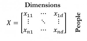
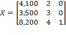
[31] The achievements of all persons within a society are denoted by an

-dimensional achievement matrix

which looks as follows:
We denote the set of all possible matrices of size
by

and the set of all possible achievement matrices by

, such that

. If

, then matrix
contains achievements for
persons in
dimensions. Unless specified otherwise, whenever we refer to matrix
, we assume

. The achievements of any person
in all
dimensions, which is row
of matrix
, are represented by the
-dimensional vector

for all
. The achievements in any dimension
for all
persons, which is column
of matrix
, are represented by the
-dimensional vector

for all
. In the unidimensional context, the
dimensions considered in matrix
—which are typically assumed to be cardinal—can be meaningfully combined into a well-defined overall achievement or resource variable for each person
, which is denoted by

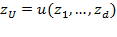
. One possibility, from a welfarist approach, would be to construct each person’s welfare from her vector of achievements using a utility function
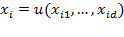
.
[32] Another possibility is that each dimension
refers to a different source of income (labour income, rents, family allowances, etc.). Then, one can construct the total income level for each person
as the sum of the income level obtained from each source, that is

. Alternatively, each dimension
can be measured in the quantity of a good or service that can be acquired in a market. Then, one can construct the total consumption expenditure level for each person
as the sum of the quantities acquired at market price, that is
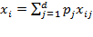
, where

, the price of commodity

is used as its weight. In any of these three cases, the achievement matrix
is reduced to a vector
containing the welfare level or the resource variables of all
persons. In other words, the distinctive feature of the unidimensional approach is not that it necessarily considers only one dimension, but rather that it maps
multiple dimensions of poverty assessment into a
single dimension using a common unit of account.
[33]
2.1.1 Identification of the Income Poor
Since Sen (1976), the measurement of poverty has been conceptualised as following two main steps:
identification of who the poor are and
aggregation of the information about poverty across society. In unidimensional space, the identification of who is poor is relatively straightforward: the poor are those whose overall achievement or resource variable falls below the poverty line

, where the subscript

simply signals that this is a poverty line used in the unidimensional space. Analogous to the construction of the resource variable, the poverty line can be obtained aggregating the minimum quantities or achievements

considered necessary in each dimension. It is assumed that such quantities or levels are positive values, that is

.
[34] These minimum levels are collected in the
-dimensional vector

. If the overall achievement is the level of utility, a utility poverty line needs to be set as
.
[35] On the other hand, when the overall achievement is total income or total consumption expenditure, the poverty line is given by the estimated cost of the basic consumption basket

—or some increment thereof.
[36] Then, given the person’s overall resource value or utility value and the poverty line, we can define the identification function as follows:

identifies person
as poor if

, that is, whenever the resource or utility variable is below the poverty line, and

identifies person
as non-poor if

. We denote the number of unidimensionally poor persons in a society by

and the set of poor persons in a society by

, such that
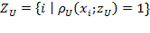
.
2.1.2 Aggregation of the Income Poor
In terms of aggregation, a variety of indices have been proposed.
[37] Among them, the Foster, Greer and Thorbecke or FGT (1984) family of indices has been the most widely used measures of poverty by international organizations such as the World Bank and UN agencies, national governments, researchers, and practitioners.
[38] For simplicity, we assume the unidimensional variable
to be income. Building on previous poverty indices including Sen (1976) and Thon (1979), the FGT family of indices is based on the normalized income gap—called the ‘poverty gap’ in the unidimensional poverty literature—which is defined as follows: Given the income distribution

, one can obtain a
censored income distribution

by replacing the values above the poverty line
by the poverty line value
itself and leaving the other values unchanged. Formally,

if
and

if
. Then, the normalized income gap is given by:

The normalized income gap of person
is her income shortfall expressed as a share of the poverty line. The income gap of those who are non-poor is equal to 0.
[39] The individual income gaps can be collected in an
-dimensional vector
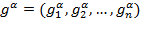
. Each

element is the normalized poverty gap raised to the power

and it can be interpreted as a measure of
individual poverty where

is a ‘poverty aversion’ parameter. The class of FGT measures is defined as
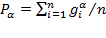
, thus

can be interpreted as the average poverty in the population. The FGT measures can also be expressed in a more synthetic way as

, where

is the mean operator and thus

denotes the average or mean of the elements of vector

. This presentation of the FGT indices is useful in understanding the AF class (Alkire and Foster 2011a). Within the FGT measures, three measures, associated with three different values of the parameter
, have been used most frequently. The deprivation vector

, for

, replaces each income below the poverty line with 1 and replaces non-poor incomes with 0. Its associated poverty measure

is called the headcount ratio, or the mean of the deprivation vector. It indicates the proportion of people who are poor, also frequently called the incidence of poverty.
[40] The normalized
gap vector

, for

, replaces each poor person’s income with the normalized income gap and assigns 0 to the rest. Its associated measure

, the poverty gap measure, reflects the average depth of poverty across the society. The squared gap
vector

for

, replaces each poor person’s income with the squared normalized income gap and assigns 0 to the rest. Its associated measure—the squared gap or distribution sensitive FGT—is

; it emphasizes the conditions of the poorest of the poor as Box 2.1 explains. The FGT measures satisfy a number of properties, including a subgroup decomposability property that views overall poverty as a population-share weighted average of poverty levels in the different population subgroups.
[41] As noted by Sen (1976), the headcount ratio violates two intuitive principles: (1) monotonicity: if a poor person’s resource level falls, poverty should rise and yet the headcount ratio remains unchanged; (2) transfer: poverty should fall if two poor persons’ resource levels are brought closer together by a progressive transfer between them, and yet the headcount ratio may either remain unchanged or it can even go down. The poverty gap measure satisfies monotonicity, but not the transfer principle; the

measure satisfies both monotonicity and the transfer principle.
[42]
Box 2.1. A numerical example of the FGT measures
A simple example
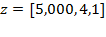
[43] can clarify the method and these axioms, and will also prove useful in linking the Alkire and Foster methodology (fully described in Chapter 5) to its roots in the FGT class of poverty measures. Consider four persons whose incomes are summarized by vector

and the poverty line is

. The headcount ratio

: Consider first the case of
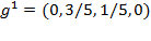
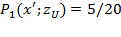
. Each gap is replaced by a value of 1 if the person is poor and by a value of 0 if non-poor. The deprivation vector is given by:

, indicating that the second and third persons in this distribution are poor. The mean of this vector—the

measure—is one half:
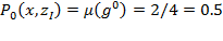
, indicating that 50% of the population in this distribution is poor. Undoubtedly, it provides very useful information. However, as noted by Watts (1968) and Sen (1976), the headcount ratio does not provide information on the depth of poverty nor on its distribution among the poor. For example, if the third person became poorer, experiencing a decrease in her income so that the income distribution became

, the
measure would still be one half; that is, it violates monotonicity. Also, if there was a progressive transfer between the two poor persons, so that the distribution was

, the
measure would not change, violating the transfer principle. This has policy implications. If this was the official poverty measure, a government interested in maximising the impact of resources on poverty reduction would have an incentive to allocate resources to the least poor, that is, those who were closest to the poverty line, leaving the lives of the poorest of the poor unchanged. The poverty gap

(or FGT-1): Here

Each gap is raised to the power
, giving the proportion in which each poor person falls short of the poverty line and

if the person is non-poor. The normalized gap vector is given by
. The

measure is the mean of this vector.
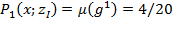
, indicates that the society would require an average of 20% of the poverty line for each person in the society to remove poverty. In fact, $4 is the overall amount needed in this case to lift both poor persons above the poverty line. Unlike the headcount ratio
, the
measure
is sensitive to the depth of poverty and satisfies monotonicity. If the income of the third person decreased so we had

the corresponding normalized gap vector would be
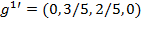
, so
. Clearly,
. Indeed, all measures with

satisfy monotonicity. However, a transfer to an extremely destitute person from a less poor person would not change
, since the decrease in one gap would be exactly compensated by the increase in the other. By being sensitive to the depth of poverty (i.e. satisfying monotonicity), the
measure does make policy makers want to decrease the average depth of poverty as well as reduce the headcount. But because of its insensitivity to the distribution among the poor,
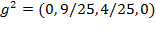
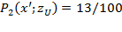
does not provide incentives to target the very poorest, whereas the FGT-2 measure does. The Squared Poverty Gap

(or FGT-2): When we set
, each normalized gap is squared or raised to the power
. The squared gap vector in this case is given by:
. By squaring the gaps, bigger gaps receive higher weight. Note for example that while the gap of the second person (

) is three times bigger than the gap of the third person (

), the squared gap of the second person (

) is nine times bigger than the gap of the third person (

). The mean of the
vector—the
measure—is
. The
measure is sensitive to the depth of poverty: if the income of the third person decreases one unit such that
, the squared gap vector becomes
, increasing the aggregate poverty level to
). It is also sensitive to the distribution among the poor: if there is a transfer of $1 from the third person to the second one, so
becomes

, the squared gap vector becomes
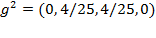
, decreasing the aggregate poverty level to
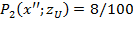
. Squaring the gaps has the effect of emphasising the poorest poor and providing incentives to policy makers to address their situation urgently. All measures with

satisfy the transfer property
2.2 Notation and Preliminaries for Multidimensional Poverty Measurement
We now extend the notation to the multidimensional context. We represent achievements as
dimensional achievement matrix
, as in the unidimensional framework described in section 2.1. We make two practical assumptions for convenience. We assume that the achievement of person
in dimension
can be represented by a non-negative real number, such that
for all
and
. Also, we assume that higher achievements are preferred to lower ones.
[44] In a multidimensional setting, in contrast to a unidimensional context, the considered
achievements may not be combinable in a meaningful way into some overall variable. In fact, each dimension can be of a different nature. For example, one may consider a person’s income, level of schooling, health status, and occupation, which do not have any common unit of account. As in the unidimensional case, we allow the population size of a society to vary, and we assume
to denote a fixed set (and number) of dimensions.
[45] We denote the set of all possible matrices of size
by
and the set of all possible achievement matrices by
, such that
. If
, then matrix
contains achievements for
persons and a fixed set of
dimensions. Unless specified otherwise, whenever we refer to matrix
, we assume
. The achievements of any person
in all
dimensions, which is row
of matrix
, are represented by the
-dimensional vector
for all
. The achievements in any dimension
for all
persons, which is column
of matrix
, are represented by the
-dimensional vector
for all
. In multidimensional analysis, each dimension may be assigned a weight or deprivation value based on its relative importance or priority. We denote the relative weight attached to dimension
by

, such that

for all
. The weights attached to all
dimensions are collected in a vector
. For convenience we may restrict the weights such that they sum to the total number of considered dimensions, that is:

Alternatively, weights may be normalized; in other words, the weights sum to one:

.
[46]
2.2.1 Identifying Deprivations
A common first step in multidimensional poverty assessment in several of the methodologies reviewed in Chapter 3, as well as in the Alkire and Foster (2007, 2011a) methodology, requires defining a threshold in
each dimension. Such a threshold is the minimum level someone needs to achieve in that dimension in order to be non-deprived. It is called the dimensional
deprivation cutoff. When a person’s achievement is strictly below the cutoff, she is considered deprived. We denote the deprivation cutoff in dimension
by
; the deprivation cutoffs for all dimensions are collected in the
-dimensional vector
. We denote all possible
-dimensional deprivation cutoff vectors by

. Any person
is considered deprived in dimension
if and only if

. For several measures reviewed in Chapter 3, and for the AF method, it will prove useful to express the data in terms of deprivations rather than achievements. From the achievement matrix
and the vector of deprivation cutoffs

, we obtain a deprivation matrix
(analogous to the deprivation vector in the unidimensional context) whose typical element

whenever

and

, otherwise, for all
and for all
. In other words, if person
is deprived in dimension
, then the person is assigned a deprivation status value of 1 and 0, otherwise. Thus, matrix

represents the deprivation status of all
persons in all
dimensions in matrix
. Vector

represents the deprivation status of person
in all dimensions and vector

represents the deprivation status of all persons in dimension
. From the matrix
one can construct a deprivation score

for each person
such that
. In words,
denotes the sum of
weighted deprivations suffered by person
.
[47] In the particular case in which weights are equal and sum to the number of dimensions, the score is simply the number of deprivations or deprivation counts that the person experiences. Whenever weights are unequal but sum to the number of dimensions, person
 deprivation score
 is defined as the sum of her weighted deprivation counts. The deprivation scores are collected in an
-dimensional column vector

. On certain occasions, it will be useful to use the deprivation-cutoff-
censored achievement matrix 
which is obtained from the corresponding achievement matrix
in
, replacing the non-deprived achievements by the corresponding deprivation cutoff and leaving the rest unchanged. We denote the
 th
th element of

by

. Then, formally,

if
and

, otherwise. In this way, all achievements greater than or equal to the deprivation cutoffs are ignored in the censored achievement matrix. When data are cardinally meaningful for all
and all
, and

, in other words, when all the achievements take non-negative values and the deprivation cutoffs take strictly positive values, one can construct dimensional gaps or shortfalls from the censored achievement matrix

as:
[48] 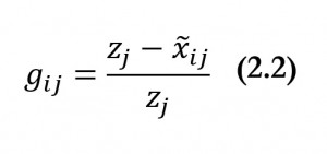
Each

or normalized gap, expresses the shortfall of person
in dimension
as a share of its deprivation cutoff. Naturally, the gaps of those whose achievement

is above the corresponding dimensional deprivation cutoff
are equal to 0. Generalizing the above, the individual normalized gaps can be collected in an
dimensional matrix
where each

element is the normalized gap defined in (2.2) raised to the power
; such normalized gaps can be interpreted as a measure of
individual deprivation in dimension
. When
, we have the
deprivation matrix already defined. When
, we have the
matrix of normalized gaps, and when
, we have the
matrix of squared gaps. Analogous to the FGT measures,
is a deprivation aversion parameter.
2.2.2 Identification and Aggregation in the Multidimensional Case
Sen’s (1976) steps of
identification of the poor and
aggregation also apply to the multidimensional case. It is clear that the identification of who is poor in the unidimensional case is relatively straightforward. The poverty line dichotomizes the population into the sets of poor and non-poor. In other words, in the unidimensional case, a person is poor if she is deprived. However, in the multidimensional context, the identification of the poor is more complex: the terms ‘deprived’ and ‘poor’ are no longer synonymous. A person who is deprived in any particular dimension may not necessarily be considered poor. An identification method, with an associated identification function, is used to define who is poor. We denote the identification function by

, such that

identifies person
as poor and

identifies person
as non-poor. Analogous to the unidimensional case, we denote the number of multidimensionally poor people in a society by

and the set of poor persons in a society by

, such that
. It could be the case that the identification method is based on some ‘exogenous’ variable, in that it is a variable not included in achievement matrix

For example, the exogenous variable could be being beneficiary of some government programme or living in a specific geographic area. One may also define an identification method based on one particular dimension
of matrix
. One may consider the corresponding normative cutoff
to identify the person as poor, in which case the function is

, or one may consider a relative cutoff identifying as poor anyone who is below the median or mean value of the distribution, in which case the function is

. Alternatively, identification may be based on the whole set of achievements not necessarily considering dimensional deprivation cutoffs but rather the relative position of each person on the aggregate distribution

. There are many different ways of identifying the poor in the multidimensional context. A particularly prevalent set of methods consider the person’s vector of achievements and corresponding deprivation cutoffs, such that

identifies person
as poor and

identifies person
as non-poor.
[49] Within this specification of the identification function, at least two approaches can be followed. An approach closely approximating unidimensional poverty is the ‘aggregate achievement approach’, which consists of applying an aggregation function to the achievements across dimensions for each person to obtain an overall achievement value. The same aggregation function is also applied to the dimensional deprivation cutoffs to obtain an aggregate poverty line. As in the unidimensional case, a person is identified as poor when her overall achievement is below the aggregate poverty line. Another method, which we refer to as ‘censored achievement approach’, first applies deprivation cutoffs to identify whether a person is deprived or not in each dimension and then identifies a person considering only the deprived achievements. The ‘counting approach’ is one possible censored achievement approach, which identifies the poor according to the number (count) of deprivations they experience. Note that ‘number’ here has a broad meaning as dimensions may be weighted differently. Chapter 4 and the AF method (Ch 5-10) use a counting approach. When the scale of the variables allows, other identification methods could be developed using the information on the deprivation gaps.
In counting identification methods, the criterion for identifying the poor can range from ‘union’ to the ‘intersection’. The union criterion identifies a person as poor if the person is deprived in
any dimension, whereas the intersection criterion identifies a person as poor only if she is deprived in
all considered dimensions. In between these two extreme criteria there is room for intermediate criteria. Many counting-based measurement exercises since the mid-1970s have used intermediate criteria (see Chapter 4). The AF methodology formally incorporated it into an axiomatic framework.
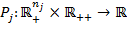
[50] Once the identification method has been selected, the aggregation step requires selecting a poverty index, which summarizes the information about poverty across society. A poverty index is a function

that converts the information contained in the achievement matrix
and the deprivation cutoff vector

into a real number. We denote a poverty index as

. An identification and an aggregation method that are used together constitute what we call a multidimensional poverty methodology, and we denote it as

. It will prove useful to introduce notation for two further partial indices related to the overall poverty index
. Each of them offers information on different ‘slices’ of the achievement matrix
as analysed by the corresponding multidimensional poverty methodology
; that is, the partial indices are dependent on the selected identification and aggregation methods. One of these partial indices is the poverty level of a particular subgroup within the total population, denoted as

, where

is the achievement matrix of this particular subgroup

(which could be people of a particular ethnicity, for example) contained in matrix
. Visually, this partial index is based on a horizontal slice of the achievement matrix
(i.e. a set of rows). The other partial index is a function of the
post-identification dimensional deprivations, denoted as

, where, as stated above, vector
represents the achievements in dimension
for all
persons and
is the deprivation cutoffs vector.
[51] This is precisely why the full vector of deprivation cutoffs
is an argument of the index and not just the particular deprivation cutoff
. Recall that under some identification methods, it is possible to have some people who experience deprivations but are not identified as poor (for example, when a counting approach is used with an identification strategy that it is not union). In such cases, their deprivations will not be considered in the poverty measure and therefore will not be considered in this partial index either. In a visual way, this partial index is based on a vertical slice of the achievement matrix
(i.e. a column). These two partial indices will be used when introducing the different principles of multidimensional poverty measures in section 2.5.3. As we shall see, although identification and aggregation have, since Sen (1976), usually been recognized as key steps in poverty measurement, some methods in the multidimensional context do not follow these steps. We will clarify this in Chapter 3.
2.2.3 The Joint Distribution
Throughout this book we will frequently refer to the
joint distribution in contrast to the
marginal distribution and we will also use the expression
joint deprivations. The concept of a joint distribution comes from statistics where it can be represented using a joint cumulative distribution function.
[52] The relevance of the joint distribution in multidimensional analysis was articulated by Atkinson and Bourguignon (1982), who observed that multidimensional analysis was
intrinsically different because there could be identical dimensional marginal distributions but differing degrees of interdependence between dimensions.
[53] In this book we treat the achievement matrix
as a representation of the joint distribution of achievements. Each row contains the (vector of) achievements of a given person in the different dimensions, and each column contains the (vector of) achievements in a given dimension across the population. From that matrix, considered with deprivation cutoffs, it is possible to obtain the proportion of the population who are simultaneously deprived in different subsets of
dimensions. In other words, it is possible to obtain the proportion of people who experience each possible profile of deprivations. This is visually clear in the deprivation matrix
, which represents the joint distribution of deprivations. The higher order matrices
and
obviously offer further information regarding the joint distribution of the depths of deprivations. The importance of considering the joint distribution of achievements, which in turn enables us to look at joint deprivations, is best understood in contrast with the alternative of looking at the
marginal distribution of achievements, and, thus, the
marginal deprivations. The marginal distribution is the distribution in one specific dimension without reference to any other dimension.
[54] The marginal distribution of dimension
is represented by the column vector

. From the marginal distribution of each dimension, it is possible to obtain the proportion of the population deprived with respect to a particular deprivation cutoff. However, by looking at only the marginal distribution, one does not know who is simultaneously deprived in other dimensions.
[55] Table 2.1 illustrates the relevance of the joint distribution in the basic case of
persons and

dimensions using a contingency table.
Table 2.1. Joint distribution of deprivation in two dimensions
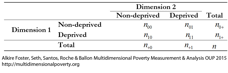
We denote the number of people deprived and non-deprived in the first dimension by

and

, respectively; whereas, the number of people deprived and non-deprived in the second dimension are denoted by

and

, respectively. These values correspond to the marginal distributions of both dimensions as depicted in the final row and final column of the table. They could equivalently be expressed as proportions of the total, in which case, for example, (

) would represent the proportion of people deprived (or the headcount ratio) in Dimension 1. The marginal distributions, however, do not provide information about the joint distribution of deprivations, which is described in the four internal cells of the table. In particular, the number of people deprived in both dimensions is denoted by

, the number of people deprived in the first but not the second dimension is denoted by

, and the number of people deprived in the second and not in the first dimension is denoted by

. We know that
people are deprived in both dimensions and the sum of
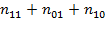
is the number of people deprived in at least one dimension. These values correspond to the joint distribution of deprivations. Consider now the case of four dimensions and four people, to see how valuable information can be added by the joint distribution. Table 2.2
[56] presents the deprivation matrix
of two hypothetical distributions,
and

. Such a matrix presents joint distributions of deprivations in a compact way and is used regularly throughout this book.
Table 2.2. Comparison of two joint distributions of deprivations in four dimensions
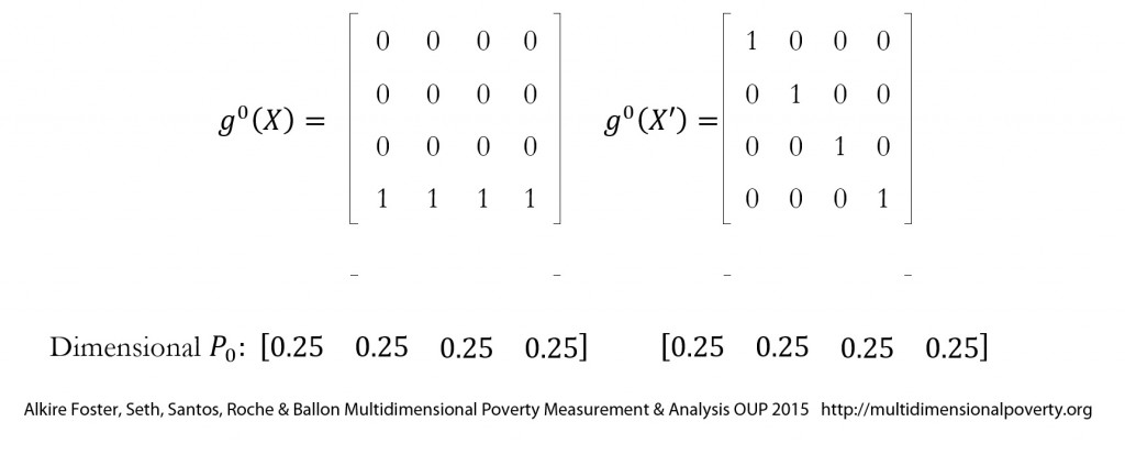
In the table, the marginal distributions of each dimension’s
are identical in deprivation matrices
and

. Thus, the proportions of people deprived in each dimension are the same in the two distributions (25%). Yet, while, in distribution

one person is deprived in all dimensions and three people experience zero deprivations, in distribution
, each of the four persons is deprived in exactly one dimension. In other words, although the marginal distributions are identical, the two joint distributions
and
are very different. We understand that multiple deprivations that are
simultaneously experienced are at the core of the concept of multidimensional poverty, and this is the reason why the consideration of the joint distribution is important. However, as we shall see, not all methodologies consider the joint distribution. In the next section, we introduce the notation for two methodologies of this type.
2.2.4 Marginal Methods
Some of the methods for multidimensional poverty assessment introduced in Chapter 3 can be called
marginal methods because they do not use information contained in the joint distribution of achievements. In other words, they ignore all information on links across dimensions. Following Alkire and Foster (2011b), a marginal method assigns the same level of poverty to any two matrices that generate the same marginal distributions. In Table 2.2, a marginal method would assign the same poverty level to distribution
(four deprivations are experienced by one person) and distribution
(each person experiences exactly one deprivation). That is, it would not be able to show whether the deprivations are spread evenly across the population or whether they are concentrated in an underclass of multiply deprived persons. Such marginal methods can also be linked to the order of aggregation while constructing poverty indices (Pattanaik et al 2012). Specifically, a measure can be obtained by first aggregating achievements or deprivations across people (column-first) within each dimension and then aggregating across dimensions, or it can be obtained by first aggregating achievements or deprivations for each person (row-first) and then aggregating across people. Only measures that follow the second order of aggregation (i.e., first across dimensions for each person and then across persons) reflect the joint distribution of deprivations (Alkire 2011: 61, Figure 7). Measures that follow the first order of aggregation fall under marginal methods of poverty measurement.
Marginal methods also include cases where achievements for different dimensions are drawn from
different data sources and/or from
different reference groups within a population—as occurred, for example, in many indicators associated with the Millennium Development Goals (MDGs). In this case, rather than having an
dimensional matrix
of achievements, one may have a ‘collection’ of vectors

, representing the achievements of

people in dimension
for all

. Note that each

vector may refer to
different sets of people such as children, adults, workers, or females, to mention a few. Suppose as before, that a deprivation cutoff
is defined. Then, we define a
dimensional deprivation index 
for dimension
by
, which assesses the deprivation profile of
people in dimension
. The deprivation index might be simply the percentage of people who are deprived in this indicator or some other statistic such as child mortality rates. Note that deprivations are clearly identified in each dimension; however, because the underlying columns of dimensional achievements are not linked, no decision on who is to be considered multidimensionally poor can be made. This is a key difference between the dimensional deprivation index
and the post-identification dimensional deprivation index

which depends on the entire deprivation cutoff vector
(and not just
) and thus captures the joint distribution of deprivations (see Section 2.2.2). Different dimensional deprivation indices

can be considered in a set, constituting the ‘dashboard approach’, or combined by some aggregation function, what is often called a ‘composite index’ (Chapter 3).
2.2.5. Useful Matrix and Vector Operations
Throughout the book, we use specific vector and matrix operations. This section introduces the technical notation covering vectors and matrices. We denote the transpose of any matrix
by

where
has the rows of matrix
converted into columns. Formally, if

and the
th element of
is written

, then

, where

is the
th element of
for all
and

. The same notation applies to a vector, with

being the transpose of
. Thus, if
is a row vector,
is a column vector of the same dimension. As stated in section 2.1 the average or mean of the elements of any vector
is denoted by

, where
. Similarly, the average or mean of the elements of any matrix
is denoted by

, where

. Later in the book we use a related expression, the so-called ‘generalized mean of order’

. Given any vector of achievements
, where

, the expression of the weighted generalized mean of order

is given by
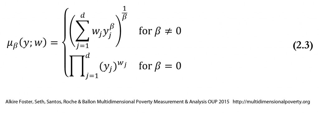
where
and
. When weights are equal,

for all
. Each generalized mean summarizes distribution

into a single number and can be interpreted as a ‘summary’ measure of well- or ill-being, depending on the meaning of the arguments

. When
for all
, we write

simply as

. When

,
reduces to the arithmetic mean and is simply denoted by

When

, more weight is placed on higher entries and
is higher than the arithmetic mean, approaching the maximum entry as
tends to

. For

more weight is placed on lower entries, and
is lower than the arithmetic mean, approaching the minimum entry as
tends to

. The case of

is known as the geometric mean and

as the harmonic mean
. Expression (2.3) is also known as a constant elasticity of substitution function, frequently used as a utility function in economics. When generalized means are computed over achievements, it is natural to restrict the parameter to the range of

giving a higher weight to lower achievements and penalizing for inequality (Atkinson 1970). Likewise when generalized means are computed over deprivations, it is natural to restrict the parameter to the range of

giving a higher weight to higher deprivations and also penalizing for inequality. Box 2.2 contains an example of generalized means.
Box 2.2. Example of generalized Means[57]
Consider two distributions
and

with the following distribution of achievements in a particular dimension:

and

. We first show how to calculate

for certain values of
and then compare two distributions with a graph where
ranges from

to
. In this example, we assume that all dimensions are equally weighted:
.
Arithmetic Mean:The arithmetic mean (
) of distribution
is:
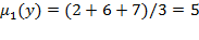
.
Geometric Mean:If
, then

is the ‘geometric mean’ and by the formula presented in (2.3) can be calculated as:
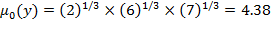
.
Harmonic Mean: If
, then
is the harmonic mean and can be calculated as:
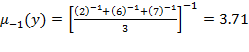
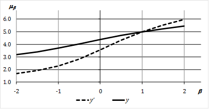
. The following graph depicts the values of the
of
and
for different values of
. Note that
when
, given that the two distributions have the same arithmetic mean. In both cases, when
, the generalized means are strictly lower than the arithmetic mean, because the incomes are unequally distributed. Note moreover that for this range,
because
has a more unequal distribution. On the other hand, for
,
as the higher incomes receive a higher weight.
Another matrix transformation that we use is
replication. A matrix is a replication of another matrix if it can be obtained by duplicating the rows of the original matrix a finite number of times. Suppose the rows of matrix

are replicated

number of times, where

. Then the corresponding replication matrix is denoted by

. notation may be used for replication of any vector
:

. We do not consider column replication, as we consider a fixed set of dimensions. Analogous We also use three types of matrices associated with particular operations: a
permutation matrix, a
diagonal matrix, and a
bistochastic matrix. A permutation matrix, denoted by

, is a square matrix with one element in each row and each column equal to 1 and the rest of the elements equal to 0. Thus the elements in every row and every column sum to one. We eliminate the special case when a permutation matrix is an ‘identity matrix’ with the diagonal elements equal to 1 and the rest equal to 0. What does a permutation matrix do? If any matrix
is pre-multiplied by a permutation matrix, then the rows of matrix
are shuffled without their elements being altered. Similarly, if any matrix
is post-multiplied by a permutation matrix, then the columns of
are shuffled without their elements being altered.
Example of Permutation Matrix: Let
. Consider

. Then
. Thus, the rows of
are merely swapped. Similarly, consider
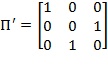
. Then


. Note that the second and the third columns have swapped their positions. The first column did not change its position because the first diagonal element in
is equal to one.
A diagonal matrix, denoted by

, is a square matrix whose diagonal elements are not necessarily equal to 0 but all off-diagonal elements are equal to 0. Let us denote the
th element of
by

. Then,

for all

. For our purposes, we require the diagonal elements of a diagonal matrix to be strictly positive or

. What is the use of a diagonal matrix? If any matrix
is post-multiplied by a diagonal matrix, then the elements in each column are changed in the same proportion. Note that different columns may be multiplied by different factors.
Example of Diagonal Matrix: Let
. Consider
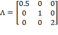
. Then


. Each element in the first column has been halved and each element in the third column has been doubled. However, the second column did not change because the corresponding element of
is equal to one.
A bistochastic matrix, denoted by

, is a square matrix in which the elements in each row and each column sum to one. If the
th element of
is denoted by

, then

for all
and

for all
. Why do we require a bistochastic matrix? If a matrix is pre-multiplied by a bistochastic matrix, then the variability across the elements of each column is reduced while their average or mean is preserved. Note that if a diagonal element in a bistochastic matrix is equal to one, the achievement vector of the corresponding person remains unaffected. If the bistochastic matrix is a permutation matrix or an identity matrix, then the variability remains unchanged.
Example of Bistochastic Matrix: Let
. Consider
. Then
. The bistochastic matrix equalizes the achievements across its elements.
2.3 Scales of Measurement: Ordinal and Cardinal Data
An important element of the framework in multidimensional poverty measurement relates to the scales of measurement of the indicators used. Scales of measurement are key because they affect the kind of
meaningful operations that can be performed with indicators. In fact, as we will observe, certain types of indicators may not allow a number of operations and thus cannot be used to generate certain poverty measures. What does
scale of measurement refer to exactly? Following Roberts (1979) and Sarle (1995), we define a scale of measurement to be a particular way of assigning numbers or symbols to assess certain aspects of the empirical world, such that the relationships of these numbers or symbols replicate or represent certain observed relations between the aspects being measured. There are different classifications of scales of measurement. In this book, we follow the classification introduced by Stevens (1946) and discussed in Roberts (1979). Stevens’ classification is consistent with Sen (1970, 1973), which analysed the implications of scales of measurement for welfare economics, distributional analysis, and poverty measurement, and it has largely stood the test of time.
[58] Stevens’ (1946) classification relies on four key concepts: assignment rules, admissible transformations, permissible statistics, and meaningful statements. First, the defining feature of a scale is the
rule or basic empirical operation that is followed for assigning numerals, as elaborated below. Second, each scale has an associated set of
admissible mathematical transformations such that the scale is preserved. That is, if a scale is obtained from another under an admissible transformation, the rule under the transformed scale is the same as under the original one. Third, a
permissible statistic
refers to a statistical operation that when applied to a scale, produces the same result as when it is applied to the (admissibly) transformed scale. While the word ‘permissible’
may sound rather strong, it is justifiable under the premise that ‘one should only make assertions that are invariant under admissible transformations of scale’ (Marcus-Roberts and Roberts 1987, 384).
[59] Fourth, a statement is called
meaningful if it remains unchanged when all scales in the statement are transformed by admissible transformations (Marcus-Roberts and Roberts 1987: 384).
[60] Stevens (1946) considered four basic empirical operations or rules that define four types of scales: equality, rank-order, equality of intervals, and equality of ratios. Following them, he defined four main types of scales: nominal, ordinal, interval, and ratio. Stevens' classification is not exhaustive. For example, it only applies to scales that take real values and which are regular.
[61] Also, note that alternative terms are sometimes used for some of Stevens’ types. For example, nominal scales are sometimes referred to as categorical scales. Table 2.3 lists the scale types mentioned above from ‘weakest’ to ‘strongest’ in the sense that interval and ratio scales contain much more information than ordinal or nominal scales. The column that presents the rule defining each scale type is cumulative in the sense that a rule listed for a particular scale must be applicable to the scales in rows preceding it. The column that lists the permissible statistics is also cumulative in the same sense. In contrast, the column that lists the admissible transformations goes from general to particular: the particular operation listed in a row is included in the operation listed above. We now introduce each scale ‘type’. The scale pertains to an indicator used to measure dimension
. The term ‘indicator
’ denotes the indicator of dimension
. Achievements in indicator
across the population are represented by vector

, where
is the achievement of person
in the

indicator. Indicator
is said to be
nominal or
categorical if the scale is based on mutually exclusive categories, not necessarily ordered. Nominal variables are frequently called
categorical variables. The rule or basic empirical operation behind this type of scale is the determination of equality among observations. A nominal scale is ‘the most unrestricted assignment of numerals. The numerals are used only as labels or type numbers, and words or letters would serve as well’ (Stevens 1946: 678). That is, numbers assigned to the various achievement levels in this domain are simply placeholders. Stevens introduces two common types of nominal variables. One uses ‘numbering’ for identification, such as the identification number of each household in a survey or the line number of individuals living within a household. The other uses numbering for a classification, such that all members of a social group (ethnic, caste, religion, gender, or age) or geographical regions (rural/urban areas, states, or provinces) are assigned the same number. The first type of nominal variable is simply a particular case of the second. There is a wide range of admissible transformations for this type of scale. In fact, any transformation that substitutes or permutes values between groups, that is, any one-to-one substitution function

such that

for all
, will leave the scale form invariant. Given that in a nominal variable, the different categories do not have an order, neither arithmetic operations nor logical operations (aside from equality) are applicable. In terms of relevant statistics, if the nominal variable is simply an identifier, then only the number of categories is a relevant statistic; if the nominal variable contains several cases in each category, then the mode and contingency methods can be implemented, as can hypotheses tests regarding the distribution of cases among the classes (Stevens 1946: 678–9). Indicator
is said to be
ordinal if the order matters but not the differences between values. The rule or basic empirical operation behind this type of scale is the determination of a rank order. Categories can be ordered in terms of ‘greater’, ‘less’, or ‘equal’ (or ‘better’, ‘worse’, ‘preferred’, ‘not preferred’). Admissible transformations consist of any order-preserving transformation, that is, any strictly monotonic increasing function
such that

for all
, as these will leave the scale form invariant. Thus, admissible transformations include logarithmic operation, square root of the values (nonnegative), linear transformations, and adding a constant or multiplying by another (positive) constant. Examples of ordinal scales are preference orderings over various categories, or subjective rankings. Given that the true intervals between the scale points are unknown, arithmetic operations are meaningless (because results will change with a change of scale), but logical operations are possible. For example, we can assert that someone reporting a health level of four feels ‘better’ than someone reporting a health level of ‘three’, who in turn feels better than a ‘two’, but we cannot assert whether the difference between level three and four is the same as the difference between level two and three. Nevertheless, some statistics are applicable to ordinal variables, namely, the number of cases, contingency tables, the mode, median, and percentiles.
[62] Statistics such as mean and standard deviation cannot be used. Clearly, an ordinal variable is a nominal variable but the converse is not true. Ordinal and nominal (or categorical) variables are also sometimes referred to as qualitative variables.
Unordered categorical variables—such as eye colour—are not relevant for the construction of poverty measures. Relevant categorical variables are those that can be exhaustively and non-trivially partitioned into at least two sets according to some exogenous condition, and in which those sets can be arranged in a complete ordering. There will be fewer sets than there are categorical responses, or else the original variable would already have been ordinal. If a set contains multiple elements, it may not be possible to rank those elements against one another. Hence the resulting construction would be a ‘semi-order’ (Luce 1956) or ‘quasi-order’ (Sen 1973). Additionally, it may be possible to distinguish set(s) that are considered to be adequate achievements from those that are inadequate, forming a ‘weak order’, that is, some pairs of responses can be ranked as ‘preferred to’ and some others cannot be ranked.
[63] For example, because it is difficult to assess whether it is better to have access to a public tap than to a borehole or a protected well as sources of drinkable water, the Millennium Development Goal indicator considers all three of them to be adequate sources of drinkable water (unrankable). Similarly, while one cannot rank access to an unprotected spring versus access to rainwater, both sources are considered inadequate by MDG standards. A variable thus constructed is often called an ‘ordered categorical’; we might also call the variables obtained as a weak order of categories in a nominal variable, a ‘weak-ordinal’ variable. Admissible transformations of weak ordinal variables include any transformations that partition the categorical variables into the relevant sets (safe water sources) in the same order; any apparent ordering of elements within the relevant sets can vary freely. Indicator
is said to be of
interval scale if the rule or basic empirical operation behind its scale is the determination of equality of intervals or differences. Importantly, interval scales do not have a predefined zero point. The admissible transformations of interval scale consist of the linear transformation

(with

), as this preserves the differences between categories. While the
difference between two values of an interval-scale variable is meaningful, the ratios are not. The most cited example in this literature refers to two temperature scales: Celsius (
oC) and Fahrenheit (
oF). While the difference between 15
oC and 20
oC is the same as the difference between 20
oC and 25
oC, one cannot say that 20
oC is twice as hot as 10
oC because 0
oC does not mean ‘no temperature’. That is, the Celsius scale (and Fahrenheit scale) lack a natural zero. Also, the difference between 15
oC and 20
oC and between 20
oC and 25
oC is also precisely the same if measured in Fahrenheit (59
oF and 68
oF vs
. 68
oF and 77
oF) although the value of the difference is nine rather than five degrees. An interval scale allows addition and subtraction and the computation of most statistics, namely, number of cases, mode, contingency correlations, median, percentiles, mean, standard deviation, rank-order correlation, and product-moment correlation, but it is not meaningful to compute the coefficient of variation or any other ‘relative’ measure. In multidimensional poverty measurement, one indicator that is usually of interest is the z-score of under 5-year-old children’s nutritional achievement. We consider a nutritional z-score to be of interval-scale type. Box 2.3 provides a more detailed explanation of how to compute z-scores. Z-scores range from negative to positive values, spaced in (the reference population’s) standard deviation units, and the zero value means that the child’s nutritional achievement is at the median of what is considered a healthy population. Indicator
is said to be of
ratio scale if the rule or basic empirical operation behind its scale is the determination of equality of ratios. Such a rule requires the scale to have a ‘natural zero’, namely the value 0 means ‘no quantity’ of that indicator. In other words, the value 0 is the absolute lowest value of the variable. Admissible transformations of interval-scale variables consist of functions such as

(with
), as this preserves the ratio differences. Examples of ratio-scale variables are age, height, weight, and temperature in Kelvin, as 0
o Kelvin means ‘no temperature’; 200 pounds is twice as much as 100 pounds, sixty years as thirty years and so on. Ratio-scale variables allow statements such as ‘a value is twice as large as another’, and they allow any type of mathematical operation, as well as the computation of any statistic (number of cases, mode, contingency correlations, median, percentiles, mean, standard deviation, rank-order correlation, product-moment correlation, and coefficient of variation). Interval- and ratio-scale variables constitute what are commonly referred to as
cardinal variables. It is interesting to observe that in the order presented, from nominal to ratio scales, the admissible transformations become more restricted but the meaningful statistics become more unrestricted, ‘suggesting that in some sense the data values carry more information’ (Velleman and Wilkinson 1993: 66). Stevens (1959, 24) provided an insightful example of how measurement can progress from weaker to stronger scales. Early humans probably could only distinguished between cold and warm and thus used a nominal scale. Later, degrees of warmer and colder had been introduced and so the use of an ordinal scale gained prominence. The introduction of thermometers led to the use of an interval scale. Finally, the development of thermodynamics led to the ratio scale of temperature by introducing the Kelvin scale.
Box 2.3. Children’s nutritional z-scores
The nutritional status of children under 5 years old is assessed with three anthropometric indicators: weight-for-age, also called ‘underweight’; weight-for-height, also called ‘wasting’; and height-for-age, also called ‘stunting’. The indicators are constructed as follows. The World Health Organization has measured the height and weight of a reference population of children from different ethnicities, which is considered to constitute a standard of well nourishment (WHO 2006). From that population, a distribution of weights according to each age, a distribution of heights according to each age, and a distribution of height according to each weight are obtained. Each of these are discriminated by gender. How is a child’s nutrition assessed? Let us consider the case of the weight-for-age (

) indicator. Once the weight and age of the child have been documented, this information can be expressed in her weight-for-age z-score. This is computed as the child’s observed weight minus the median weight of children of the same sex and age in the reference population, divided by the standard deviation of the reference population. That is:
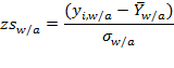
where

is the z-score of weight-for-age,

is the observed weight of child
,

is the median weight of children of the same sex and age as child
in the reference population (healthy children), and

is the standard deviation of the weight of children of that age in the reference population. The z-scores for weight-for-height (

) and height-for-age (

) are computed in an analogous way. Thus,
for all
and all

,

and
. Thus, for example, suppose 14-month-old Anna weighs 8.3 kilograms. The median weight in the reference population of children of that age is 9.4 and the standard deviation is 1.
* Thus, the z-score of Anna is

, meaning that Anna is about one standard deviation below the median weight of healthy children. It is considered that children with z-scores that are more than two standard deviations below the median of the reference population suffer moderate undernutrition, and, if their z-score is more than three standard deviations below, they suffer severe undernutrition (underweight, wasting, or stunting, correspondingly). Children with a z-score of weight-for-height above

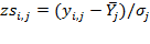
standard deviations above the median are considered to be overweight (WHO 1997). An alternative way to assess the nutritional status of children is to use percentiles rather than z-scores, but z-scores present a number of advantages. Most importantly, they can be used to compute summary statistics such as a mean and standard deviation, which cannot be meaningfully done with percentiles (O’Donnell et al. 2008). Note that if we take a linear transformation of the z-score for weight-for-age such that
, where

and
, then

. Note that the difference
(or
) has the same implication as the difference
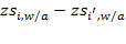
. This equivalence would hold for any linear transformation, exhibiting the characteristics of an interval-scale indicator.
*These values were taken from WHO’s reference tables: http://www.who.int/childgrowth/standards/sft_wfa_girls_z_0_5.pdf
Having introduced the scales of measurement, it is worth making a few clarifications regarding other frequently-mentioned types of indicators. First, Stevens' classification makes no reference to
continuous versus
discrete variables, for example. Continuous variables can take any value on the real line within a range. Discrete variables, in contrast, can only take a finite or countably infinite number of values.
[64] Ordinal variables are discrete variables, but cardinal ones (interval and ratio scale) can be either discrete or continuous.
[65] Second, note that
count variables such as counts of publications, number of children in a household, or number of chickens, are particular cases of ratio-scale variables (Stevens 1946), such that the only admissible transformation is the identity function, i.e.

. Roberts (1979) refers to the counting scale type as an
absolute scale. Third,
dichotomous (also called binary) variables can be of different scales, depending on the meaning of their categories. When the two values simply refer to unordered, mutually exclusive categories, such as being male or female, the variable is of nominal scale. When there is an order between the categories, such as being deprived or not in a specific dimension, the variable is
cardinal. If the two values refer to having or lacking the same thing, such as a fully functional method for wood smoke ventilation, the variable may be interpreted as of ratio scale.
[66] Fourth, the reader may wonder where do
Likert scales—introduced by Likert (1932) and often used in social sciences—fit? Likert scales are obtained from responses to a set of (carefully phrased) statements to which each respondent expresses her level of agreement on a scale such as one to five: strongly disagree, disagree, neutral, agree, or strongly agree. Each statement and its responses are known as a Likert item. A Likert scale is obtained by summing or averaging the responses to each item so that a score is acquired for each person. Likert scales are frequently treated as interval scales, under the assumption (at times empirically verified) that there is an equal distance between categories (Brown 2011; Norman 2010). Thus, descriptive statistics (like means and standard deviations) and inferential statistics (like correlation coefficients, factor analysis, and analysis of variance) are regularly implemented with Likert scales. However, this has been criticized as being ‘illegitimate to infer that the intensity of feeling between ‘strongly disagree’ and ‘disagree’ is equivalent to the intensity of feeling between other consecutive categories on the Likert scale’ (Cohen et al. 2000, cited in Jamieson 2004: 1217). Thus, there is ongoing disagreement about whether Likert scales should be treated as ordinal scales (Pett 1997; Hansen 2003; Jamieson 2004). Often empirical psychometric tests are performed to ‘verify’ whether the assumption that the scale can be treated as cardinal holds for a particular dataset.
Stevens’ (1946) landmark work sparked a body of literature on measurement theory, which raised strong warnings regarding the applicability of statistics to different scales, including Stevens (1951, 1959), Luce (1959), and Andrews et al. (1981). This engendered an extensive and on-going debate across literatures from psychology to statistics. Some social scientists and statisticians consider that, although, in theory, certain statistics such as the mean and standard deviations are inappropriate for ordinal data, they can still be ‘fruitfully’ applied if the problem in question and data structure (and comparability, if relevant) have been tested and seem to warrant assumptions that they can be treated as interval scale. The arguments in favour of this position are interestingly articulated by Velleman and Wilkinson (1993). For example, it is stated that ‘the meaningfulness of a statistical analysis depends on the questions it is designed to answer’ (Lord 1953, Guttman 1977), that in the end ‘every knowledge is based on some approximation’ (Tukey 1961), and that ‘…if science was restricted to probably meaningful statements it could not proceed’ (Velleman and Wilkinson 1993). Another argument is that parametric methods are highly robust to violation of assumptions and thus can be implemented with ordinal data (Norman 2010). Although we acknowledge this on-going debate, in what follows we do endorse the requirement of meaningfulness—as defined above—in order to compute statistics or mathematical measures in each scale type; hence, we limit the operations with ordinal data to those that cohere with its definition and point out deviations from this. As this section suggests, the indicators’ scale and the analysts’ considered response to scales of measurement must be articulated before selecting a methodology to measure and assess multidimensional poverty. In Chapter 3, we clarify whether each method surveyed can be used with ordinal data. In general, when an indicator is of ratio scale, such as income, consumption, or expenditure (all expressed in monetary units), arithmetic operations with elements of the scale are permissible. Thus, it is meaningful to compute the normalized deprivation gaps as defined in Expression (2.2). When all considered indicators are of ratio scale, multidimensional poverty measures based on normalized deprivation gaps can be used. If the indicator is of interval scale, gaps may be redefined appropriately. When indicators are ordinal, measures based on normalized deprivation gaps are meaningless because results would vary under different admissible transformations of the indicators’ scales. The Adjusted Headcount Ratio presented in Chapters 5–10 can be meaningfully implemented using ordinal indicators, provided that issues of comparability are addressed as we will now clarify.
2.4 Comparability across People and Dimensions
The last section established the scales of measurement by which we can rigorously compare achievement levels in one variable, and the mathematical and statistical operations that can be performed on that variable. The discussion enabled us to identify the scale of measurement of each single indicator. Yet multidimensional measures seek to compare people’s achievements or deprivations across indicators, in ways that respect the scale of measurement of each indicator. This is by no means elementary. As Sen (1970) pointed out, cardinally meaningful variables may not necessarily be cardinally comparable—across people or, in multidimensional measurement, across dimensions. This section scrutinizes how these comparisons can legitimately proceed. That is, it takes a step back from the material presented thus far, to make explicit assumptions that have usually been implicit in work on multidimensional poverty measurement.
The issue of comparability across dimensions raised in this section has potentially significant empirical implications for quantitative methods beyond measurement. For example, as Chapter 3 will show, dichotomous data are regularly used in techniques that implicitly attribute cardinal meaning and comparability to the 0-1 values from several dimensions. If, in fact, the associated deprivation values of these data differ significantly from one another, then results based on techniques that treat each variable as cardinally equivalent may be affected; such exercises should, strictly, employ the 0-w variables because it is their relative weights or deprivation values that create cardinal comparability across dimensions. Hence the issues raised in this section, in a preliminary and intuitive way at this stage, have far-reaching implications for multidimensional analyses.
Multidimensional poverty measures, like income poverty measures, entail a basic assumption that the indicators are interpersonally comparable. Additionally, counting-based measures further assume that the same deprivation score is associated with the same level of poverty for different people. This assumption implies that deprivations have been made comparable. Comparability across dimensions must be obtained in order to generate cardinally meaningful deprivation scores and associated multidimensional poverty measures. But how? Multidimensional poverty measures may contain fundamentally distinct components that are not measured in the same units and may have no natural means of conversion into a common variable.
Empirically, the mechanics by which apparent comparability has been created in counting-based measures are clear (Chapter 4). When data are dichotomous and interpersonally comparable, the application of deprivation values is understood to create cardinal comparability across dimensions. When data are ordinal or ordered categorical, deprivation cutoffs are used to dichotomize the data; and those cutoffs, together with deprivation values, establish cardinal comparability across deprivations. In the case of appropriately scaled cardinal data, comparability across deprivations is created by the weights and the deprivation cutoffs.
Let us start with the most straightforward case: the deprivation matrix. This presents dichotomous values either because the original indicator is dichotomous (access to electricity), or because a cardinal, ordinal or ordered categorical variable has been dichotomized by the application of a deprivation cutoff into two categories: deprived and non-deprived.
A policy maker seeking to ameliorate poverty should have a good understanding of the various normative principles that her chosen poverty measure embodies, just as a pilot of a plane must have a sound understanding of how a particular plane responds to different operations. If the policy maker has a good understanding of the principles embodied by alternative measures then she will be able to choose the measure most closely reflecting publicly desirable ethical principles and most appropriate for the application—just as a pilot will choose the best way to fly the plane for a particular journey.
The first set of properties requires that a poverty measure should not change under certain transformations of the achievement matrix. We refer to these as
invariance properties, which are
symmetry,
replication invariance,
scale invariance and two alternative focus properties,
poverty focus and
deprivation focus. The second set requires poverty to either increase or decrease with certain changes in the achievement matrix. We refer to these as
dominance properties, which are
monotonicity,
transfer,
rearrangement, and
dimensional transfer properties. The third set of principles relates overall poverty to either groups of people or groups of dimensions and, thus is called
subgroup properties. Other properties, that guarantee that the measure behaves within certain usual, convenient parameters, we refer to as
technical properties. Each of the four following sections provides a formal outline and intuitive interpretations of each set of properties.
2.5.1 Invariance Properties
The first invariance principle is
symmetry. Symmetry requires that each person in a society is treated anonymously so that only deprivations matter and not the identity of the person who is deprived. Hence this property is also often referred to as
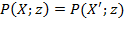
anonymity. As long as the deprivation profile of the entire society remains unchanged, swapping achievement vectors across people should not change overall poverty.
[74] This type of rearrangement can be obtained by pre-multiplying the achievement matrix by a permutation matrix of appropriate order.
Symmetry: If an achievement matrix
is obtained from achievement matrix
as

, where
is a permutation matrix of appropriate order, then
.
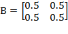
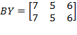
Example: Suppose the initial achievement matrix is
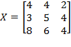
and the permutation matrix is
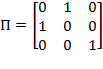
. Then:

. Note that the first and the second person (rows) in matrix
have swapped their positions. However, as long as the deprivation cutoffs remain unchanged, there is no reason for the level of poverty to be different for these two societies. Hence,
.
The second invariance principle,
replication invariance, requires that if the population of a society is replicated or cloned with the same achievement vectors a finite number of times, then poverty should not change.
[75] In other words, the replication invariance property requires the level of poverty in a society to be standardized by its population size so that societies with different population sizes are comparable to each other, as are societies whose populations change over time. Thus, this property is also known as the
principle of population.
[76]
Replication Invariance: If an achievement matrix
is obtained from another achievement matrix
by replicating
a finite number of times, then
.
Example: Suppose we are required to compare the level of poverty in two societies with the initial achievement matrices
and
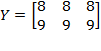
. Note that the population sizes in these societies are different. In order to make them comparable, we replicate
twice to obtain
and
thrice to obtain
. By replication invariance, we know that
and
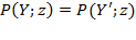
. Thus, it is equivalent comparing
to
and
to

.
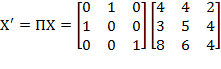
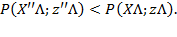
The third invariance principle,
scale invariance[77] requires that the evaluation of poverty should not be affected by merely changing the scale of the indicators. For example, if the duration of completed schooling is an indicator, then deprivation in education, thus overall poverty, should be the same regardless of whether duration is measured in years or in months, provided the deprivation cutoff is correspondingly adjusted. The scale of any indicator in an achievement matrix can be altered by post-multiplying the achievement matrix by a diagonal matrix
of appropriate order (
, the number of dimensions). If a diagonal element is equal to one, then the scale of the respective indicator does not change. The diagonal elements of
need not be the same because different indicators may have different scales and units of measurement. A weaker version of the scale invariance principle, referred to as ‘unit consistency’, has been proposed by Zheng (2007) in the context of unidimensional poverty measurement and extended to the multidimensional context by Chakravarty and D’Ambrosio (2013). This principle requires that poverty comparisons, but not necessarily poverty values, should not change if the scales of the dimensions are altered.
[78] The scale invariance property implies the unit consistency property, but the converse does not hold.
Scale Invariance: If an achievement matrix
is obtained by post-multiplying the achievement matrix
by a diagonal matrix
such that

, and the deprivation cutoff vector

is obtained from

such that

, then
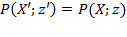
.
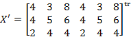
Unit
Consistency: For two achievement matrices
and

and two deprivation cutoff vectors
and

, if
, then
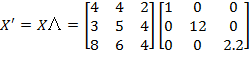
Example: Suppose the initial achievement matrix is
and the deprivation cutoff vector is

. Matrix
is post-multiplied by the diagonal matrix
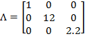
to obtain
. Similarly, vector
is post-multiplied by
to obtain
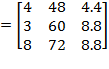
. Note that the first indicator and its deprivation cutoff did not change at all because the first diagonal element in
is 1. The second diagonal element in
is 12, as in 1 year = 12 months, and the third diagonal element in
is 2.2, as in 1 kilogram = 2.2 pounds. Scale invariance
requires that this transformation does not change overall poverty. Hence,
. Now suppose that there exists a hypothetical achievement matrix
such that
. Then, the unit consistency
property requires that the comparison does not change if both matrices and the vector

of deprivation cutoffs are multiplied by a diagonal matrix. Hence,
More formally, we say that

is obtained from

as an
equivalent representation if there exist appropriate admissible transformations

for
such that

and

for all
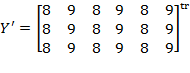
. In other words, an equivalent representation can comprise a set of admissible transformations, each of which is appropriate for each scale type, and which assigns a different set of numbers to the same underlying basic data. For example, an equivalent representation can include monotonic increasing transformations for ordinal variables, linear transformations for interval-scale variables, and proportional changes for ratio-scale variables. We now state the ordinality axiom as follows:
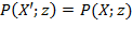
Ordinality: Suppose that
is obtained from
as an equivalent representation, then
.
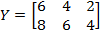
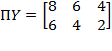
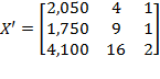
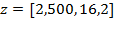
Example: Suppose the initial achievement matrix is
and the deprivation cutoff vector is
, where the first dimension is measured with a ratio-scale indicator, say income in dollars

; the second dimension is measured with an ordinal-scale indicator, say self-rated health on a scale of one to five; and the third indicator is measured with a dichotomous 0-1 variable, say access to electricity. Suppose that income is now expressed in some other currency

, such that

(note that

in this case), self-rated health is now expressed with the scale (

and

) (note that

), and access to electricity is now coded as

for no access and
for access (i.e.

). Thus matrix
obtained from
is such that
, and
, then the ordinality property requires that
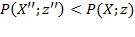
2.5.2 Dominance Properties
This section covers six principles, each of which has a stronger version and a weaker version. The stronger version requires that a poverty measure strictly moves in a particular direction, given certain transformations in the achievements of the poor. The weaker version, does not
require a poverty measure to move in a particular direction but ensures that the poverty measure does not move in the opposite (wrong) direction under certain transformations of the achievements.
[81] The first dominance principle,
monotonicity, requires that if the achievement of a poor person in a deprived dimension increases while other achievements remain unchanged, then overall poverty should decrease. Normatively, this principle considers that improvements in deprived achievements of the poor are good and should be reflected by producing a reduction in poverty. Its weaker version, referred to as weak monotonicity, ensures that poverty should not increase if there is an increase in any person’s achievement in the society.
[82]
Monotonicity: If an achievement matrix
is obtained from another achievement matrix
such that
for some pair

where

, and

for every other pair

, then
.
Weak Monotonicity: If an achievement matrix
is obtained from another achievement matrix
such that

for some pair
and
for every other pair
, then
.
Example: Suppose the initial achievement matrix is
and the deprivation cutoff vector is
. Clearly, the first person is deprived in all three dimensions and is considered poor. If matrix
is obtained from
such that
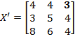
, then by the monotonicity principle,
. On the other hand, weak monotonicity requires that
; it ensures that poverty does not increase due to the increase in achievement.
The monotonicity and weak monotonicity principles are natural extensions of the analogous concepts in the unidimensional poverty analysis. However, the next principle in this category, referred to as dimensional monotonicity, is specific to the multidimensional context. This principle was introduced by Alkire and Foster (2011a). Dimensional monotonicity requires that if a poor person, who is not deprived in all dimensions, becomes deprived in an additional dimension then poverty should increase. This principle ensures that we are not only concerned with the number of poor in a society but also with the extent to which the poor are deprived in multiple dimensions—what we call the intensity of their deprivation. A measure that satisfies monotonicity also satisfies dimensional monotonicity.
Dimensional Monotonicity: If an achievement matrix
is obtained from another achievement matrix
such that

for some pair
where
and
for every other pair
, then
.
Weak Dimensional Monotonicity: If an achievement matrix
is obtained from another achievement matrix
such that
for some pair
where
and
for every other pair
, then
.
Example: Suppose the initial achievement matrix is
and the deprivation cutoff vector is
. Suppose the second person is identified as poor by some criterion but is not deprived in all dimensions. If matrix
is obtained from
by the second person becoming deprived in a principle additional dimension such that
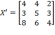
, then by dimensional monotonicity,
.
The third principle in the category of dominance principles,
transfer, is concerned with the inequality among the poor. This property has been borrowed from the multidimensional inequality measurement literature, and governs how a poverty measure should behave when the distribution of achievements among the poor becomes more or less equal while their average achievements remain the same. There are different ways of reducing inequality within a multidimensional distribution (see Marshall and Olkin 1979). We follow the approach known as
uniform majorization Kolm (1977). A uniform majorization among the poor is a transformation in which the achievements among the poor are averaged across them or, equivalently, the original bundles of achievements of poor individuals are replaced by a convex combination of them. It is worth noting that the ‘averaging’ occurs within dimensions, across people.
[83] Mathematically, this transformation is obtained by pre-multiplying the achievement matrix by a bistochastic matrix. The transfer principle requires that if an achievement matrix is obtained from another achievement matrix by reducing inequality among the poor, while the average achievement among the poor remains the same, then poverty decreases.
[84] The
weak transfer principle ensures that poverty does not increase when achievements among the poor become more equal.
Transfer: If an achievement matrix
is obtained from another achievement matrix
such that

where
is a bistochastic matrix which is not a permutation or an identity matrix and

for all

, then
.
Weak Transfer: If an achievement matrix
is obtained from another achievement matrix
such that
where
is a bistochastic matrix which is not a permutation or an identity matrix and
for all
, or
.
Example: Suppose the initial achievement matrix is
and the deprivation cutoff vector is
. The first person is indeed poor—being deprived in all three dimensions. Suppose the second person is also identified as poor by some criterion. Consider the bistochastic matrix
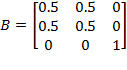
, where the achievements are distributed equally across the two poor persons so that
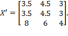
The transfer principle requires that
; whereas the weak transfer principle requires that
.
The transfer principle in the multidimensional context is similar its unidimensional counterpart, which is also concerned with the spread of the distribution. There is a second form of inequality among the poor that is only relevant in the multidimensional context, and depends on how dimensional achievements are associated across the population. This second form of inequality corresponds to the joint distribution of achievements, and was introduced by Atkinson and Bourguignon (1982): ‘in the study of multiple deprivation, investigators have been concerned with the ways in which different forms of deprivation (…) tend to be associated…’ (p. 183). Authors working on this issue have used both the term ‘correlation’ and the term ‘association’. Correlation refers to the degree of linear association between two variables, whereas association is a broader term that includes linear association and also encompasses other forms of association such as quadratic or simply rank association.
[85] Given a monotonic transformation of a variable, it is possible that while some form of association, such as rank association, remains invariant, the degree of correlation changes. Thus, here we prefer to use the broader concept of association to define the related properties. The principles that require a measure to be sensitive to the association between dimensions refer to a specific type of rearrangement of the achievements across the population that we call ‘association decreasing rearrangement’.
[86] The intuition is as follows. Imagine that originally person

is at least as well off in all dimensions as person
. Then, there is a switch in the achievement of one or more dimensions, but not in all dimensions, between the two persons such that, after the switch, person
no longer has achievements equal to or higher than person
in
all dimensions but only in some. Suppose also that the achievements of everyone else remain unchanged. Such a transformation constitutes an association-decreasing rearrangement
. Formally, given two persons
and
in

such that

for all
, if matrix
is obtained from
such that

and

for some dimension
and

for all

and all

, and
is not a permutation of
, then
is stated to be obtained from
by an association-decreasing rearrangement. The requirement that
is not a permutation of
prevents the switch from taking place in dimensions where both people have equal achievements.
Example: Suppose the initial achievement matrix is
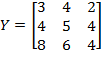
. Suppose
is obtained from
so that
. Note that the persons in the first two rows have switched their achievements in the first dimension so that the person in the first row no longer has a lower achievement than the next person in all three dimensions. Thus,
is obtained from
by an association-decreasing rearrangement. In fact, note that the achievement vectors of the first and the second person are comparable by vector dominance in
(each element in one vector is equal to or greater than the same element in the other vector) but not in
. Hence, the overall association between dimensions in
is lower.
Should poverty increase or decrease due to an association-decreasing rearrangement among the poor? One possible intuitive view is that poverty should go down or at least not increase because the association-decreasing rearrangement seems to reduce inequality among the poor. In the numerical example above, the first person was originally more deprived in all dimensions than the second person, and after the rearrangement, she is less deprived in one dimension. This was the argument provided by Tsui (2002). However, in line with Atkinson and Bourguignon (1982), Bourguignon and Chakravarty (2003) argued that the change in overall poverty should be contingent on the relation between dimensions, namely, whether they are substitutes or complements. When dimensions are thought to be substitutes for one another, poverty should not increase under the association-decreasing rearrangement. The intuition is that if dimensions are substitutes, an association-decreasing rearrangement helps both people compensate for their meagre achievements in some dimensions with higher achievements in other, a capacity that was limited for one of them before the rearrangement. When indicators are thought to be complements, poverty should not decrease under the described transfer. The intuition is that the association-decreasing rearrangement has reduced the ability of one of the persons to combine achievements and reach a certain level of wellbeing.
[88] Based on the arguments above, the following properties can be defined. As with the case of monotonicity and transfer, we may define a strong and a weak version of each of the properties.
Weak Rearrangement (Substitutes): If an achievement matrix
is obtained from another achievement matrix
by an association-decreasing rearrangement among the poor, then
.
Converse Weak Rearrangement (Complements): If an achievement matrix
is obtained from another achievement matrix
by an association-decreasing rearrangement among the poor, then
.
Strong Rearrangement (Substitutes): If an achievement matrix
is obtained from another achievement matrix
by an association-decreasing rearrangement among the poor, then
.
Converse Strong Rearrangement (Complements): If an achievement matrix
is obtained from another achievement matrix
by an association-decreasing rearrangement among the poor, then
.
The weak versions of these properties have been previously defined; the strict versions have not.
[89] Note that the properties above are applicable when the identification function uses the deprived as well as the non-deprived dimensions to identify poor people. In other words, a poor person’s identification status is allowed to change even when their achievements in non-deprived dimensions change while their achievements in the deprived dimensions remain unchanged. The rearrangement set of properties could be made more precise when the identification of the poor respects the deprivation-focus property as well as the poverty-focus property. Identification that respects deprivation focus occurs when identification is solely based on dimensions in which poor persons are deprived, not on dimensions in which poor persons are not deprived. For example, these properties cannot distinguish situations when a poverty measure satisfying the deprivation-focus property should be strictly or weakly sensitive to the joint distribution of achievements among the poor. Let us consider the following two examples where the deprivation cutoff vector is

]. In the first example, suppose the achievement matrix
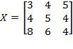
is obtained from
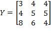
by switching the achievements between the two poor persons in the third dimension. Clearly, an association-decreasing rearrangement has taken place between the two poor persons in
, but this switch should not affect overall poverty as none of these two persons is deprived in the third dimension. In the second example, suppose
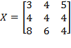
is obtained from
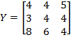
by switching the achievements between the two poor persons in the first dimension. Again, certainly an association-increasing rearrangement has taken place, but if we look at the achievements in the deprived dimensions of the two poor persons, they appear to be permutations of each other and thus overall poverty should not change. In order to make the transformations relevant in this situation, we need to ensure that the association-decreasing rearrangements occur only among the deprived dimensions of the poor. Thus, there is a need to define a new set of properties that is compatible with the deprivation-focus property, which can be done by defining the properties in terms of the censored achievement matrices. In this book, we define an additional set of new rearrangement properties by defining a transformation called
association-decreasing deprivation rearrangement among the poor. Let

and
denote the censored achievement matrices for
and
, respectively (defined in section 2.2.5 of this chapter). Consider two poor persons
and
in
such that
for all
. If matrix
is obtained from
such that
and
for some dimension
, and
for all
and all
, and
is not a permutation of
, then
is stated to be obtained from
by an association-decreasing deprivation rearrangement among the poor. The requirement of
not being a permutation of
has two analogous implications as in case of the association decreasing rearrangement. It prevents the two cases presented in the previous paragraph. Thus, it does not consider the cases where the switch of achievements between the two (poor) persons takes place in their non-deprived dimensions instead of the deprived dimension. Also, it prevents the censored deprivation vectors from being permutations of each other due to an association-decreasing rearrangement. The following example illustrates the transformation.
Example: Suppose the initial achievement matrix is
and the deprivation cutoff vector is
. Thus, the first person is deprived in three dimensions, the second person is deprived only in the two first dimensions, and the third person is non-deprived in all three dimensions. Moreover, the first person is more deprived than the second one in every dimension. The corresponding censored achievement matrix is given by
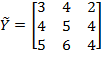
. Now, suppose
is obtained from
such that
. Note that the first and the second person have switched their achievements in the first dimension so that now the first person is no longer more deprived than the second person in all three dimensions. The corresponding censored achievement matrix is given by
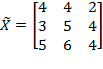
which is clearly not a permutation of
. In this case,
is said to be obtained from
by association-decreasing deprivation rearrangement among the poor.
We define the following four additional properties using the same concept of substitutability and complementarity between dimensions discussed previously, but require the association-decreasing rearrangement to take place between the deprived dimensions of the poor. Note that, due to the transformation, the set of poor remains unchanged.
Weak Deprivation Rearrangement (Substitutes): If an achievement matrix
is obtained from another achievement matrix
by an association-decreasing deprivation rearrangement among the poor, then
.
Converse Weak Deprivation Rearrangement (Complements): If an achievement matrix
is obtained from another achievement matrix
by an association-decreasing deprivation rearrangement among the poor, then
.
Strong Deprivation Rearrangement (Substitutes): If an achievement matrix
is obtained from another achievement matrix
by an association-decreasing deprivation rearrangement among the poor, then
.
Converse Strong Deprivation Rearrangement (Complements): If an achievement matrix
is obtained from another achievement matrix
by an association-decreasing deprivation rearrangement among the poor, then
.
How are deprivation rearrangement properties related to or different from the rearrangement properties? First, if a poverty measure satisfies the (converse) weak deprivation rearrangement property, then the poverty measure will satisfy the (converse) weak rearrangement property, and the converse is true as well. Also, a poverty measure that satisfies the (converse) strong deprivation rearrangement property automatically satisfies the (converse) strong rearrangement property. But a poverty measure that satisfies the (converse) strong rearrangement property does not necessarily satisfy the (converse) strong deprivation rearrangement property. Therefore, the main difference between these two set of properties lies in their strong versions. Although the rearrangement properties show technically how the change in poverty is related to association between dimensions, further research is required to understand the practicalities of rearrangement properties. Importantly, note that these properties require a uniform assumption across dimensions: either they are
all substitutes, or they are
all complements, which may be highly constraining. On the empirical side, there does not seem to be a standard procedure for determining the extent of substitutability and complementarity across dimensions of poverty. Moreover, it is not entirely clear that any interrelationships across variables must be incorporated into the overarching methodology for evaluating multidimensional poverty. Instead, the interconnections might plausibly be the subject of separate empirical investigations that supplement, but do not constitute, the underlying poverty measure. A related property, which is consistent with the ordinality property discussed in section 2.5.1, is dimensional transfer. The association-decreasing rearrangement, as well as the association-decreasing deprivation rearrangement among poor people, requires the achievements of poor people to be rearranged. However, some rearrangements, even when achievement matrices are not permutations of each other, may not alter the deprivation status of the poor and thus the corresponding deprivation matrices may either be identical or a permutation of each other. Therefore, the rearrangement properties discussed above are not useful for judging whether an ordinal poverty measure (as we discuss in Section 3.6.1) is strictly or weakly sensitive to data transformations when deprivations are transferred between poor persons. Let us show with an example how an association-decreasing rearrangement among the poor may cause no change in the deprivation matrices. Suppose two achievement matrices
and
with deprivation cutoff vector
, where
is obtained from
by an association-decreasing rearrangement among the poor. These two achievement matrices have identical corresponding deprivation matrices, such that
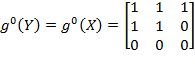
. A dimensional rearrangement among the poor is an association-decreasing rearrangement among the poor (in achievements) that is simultaneously an association-decreasing rearrangement in deprivations. In other words, the initial deprivation vectors (and achievement vectors) are ranked by vector dominance, while the final deprivation vectors (and achievement vectors) are not. The extra condition ensures that the person with a lower level of achievements is actually deprived in some dimensions in which the other person is not and that, through the rearrangement, one or more of these deprivations (but not all) are traded for non-deprived levels. More formally, let

and
denote the deprivation matrices for
and
, respectively (defined in Section 2.2.1). Consider two poor persons

and

(according to some identification method
) in
such that
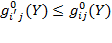
for all
. If matrix
is obtained from
such that
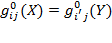
and
for some dimension
, and
for all
and all
, and
is not a permutation of
, then we define
to be obtained from
by an
dimensional rearrangement among the poor. A dimensional rearrangement among the poor does not affect the number of poor persons, and neither does a dimensional increment among the poor. This transformation can be interpreted as a progressive transfer in that it transforms an initial ‘spread’ in joint deprivations between two poor persons into a moderated situation where neither person has unambiguously more than the other. The overall achievement levels in society are unchanged, but the correlation between dimensions (and hence inequality) has been reduced. The following property requires poverty to decrease when there is a dimensional rearrangement among the poor.
Dimensional rearrangement among the poor, as defined above, covers only switches of achievements and deprivations in deprived dimensions among people who are and remain poor, and excludes permutations of corresponding deprivation matrices.
Dimensional Transfer: If an achievement matrix
is obtained from another achievement matrix
by a dimensional rearrangement among the poor, then
.
[61]
2.5.3 Subgroup Properties
The next set of principles is concerned with the link between overall poverty and poverty in different subgroups of the population, and the link between overall poverty and dimensional deprivations. The first principle—
subgroup consistency—ensures that the change in overall poverty is consistent with the change in subgroup poverty.
[91] For example, suppose the entire society is divided into two population subgroups: Group 1 and Group 2. Poverty in Group 1 remains unchanged while poverty in Group 2 decreases. One would expect overall poverty to decrease. If overall poverty did not reflect subgroup poverty, there would be an inconsistency, which would be conceptually and politically problematic. As a result, national poverty estimates would not reflect regional successes in poverty reduction. A related principle with a stronger requirement is
population subgroup decomposability. This principle requires overall poverty to be equal to a weighted sum of subgroups’ poverty, noted as
in section 2.2.2, where the weight attached to each subgroup’s poverty is the population share of that subgroup.
Suppose an achievement matrix
is divided into

subgroups, such that
and

denote, correspondingly, the achievement matrix and the population size of subgroup
, for all

, and the subgroups are mutually exclusive and collectively exhaustive:

.
Subgroup Consistency: If an achievement matrix
is obtained from the achievement matrix
such that
but
for all

, and total population, as well as subgroup population, remains unchanged, then
.
Population Subgroup Decomposability: 
Example: Suppose the initial achievement matrix is
. Let us divide
into two subgroups
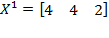
with population size

and
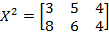
with population size

. Now, suppose

changes to
and

. We know that by the monotonicity principle,
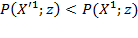
. Then the subgroup consistency principle requires that
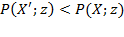
. The additive decomposability principle requires that overall poverty can be expressed as
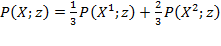
.
The population subgroup decomposability property has been one of the most attractive properties for policy analysis as it can be particularly useful for targeting and monitoring progress in different subgroups. It is worth noting that a poverty measure that satisfies population subgroup decomposability necessarily satisfies subgroup consistency. However, the converse is not true, which means subgroup consistency does not necessarily imply population subgroup decomposability. The other form of decomposition that is of tremendous relevance in the policy analysis of multidimensional poverty refers to the possibility of breaking down poverty by deprivations across dimensions among the poor. This property, called
dimensional breakdown, requires overall poverty to be equal to a weighted sum of the dimensional deprivations
after identification 
introduced in section 2.2.2. It creates a consistency between the post-identification dimensional deprivations and overall poverty.
In the particular case in which a counting approach using a union criterion is followed for identification, then
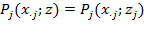
, provided the base population

for all
. In other words, the dimensional deprivation of any dimension
after identification coincides with the dimensional deprivation level before identification. In this special case, the property of dimensional breakdown coincides with the property of ‘factor decomposability’
introduced by Chakravarty, Mukherjee, and Ranade (1998) and referred to by Bossert, Chakravarty, and D’Ambrosio (2013) as ‘additive decomposability in attributes’. In other cases, dimensional breakdown is done after the identification of the poor and shows only the deprivations faced by the poor.
Dimensional Breakdown: For an
dimensional achievement matrix
,
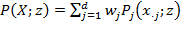
, where
is the weight attached to dimension
and
is the dimensional deprivation index after identification in dimension
.
Given that the dimensional breakdown property requires additivity in the deprivations, it is not consistent with the properties of association sensitivity in their strict form—that is, with requiring decreasing or increasing poverty under an association-decreasing rearrangement.
[92]
2.5.4 Technical Properties
Finally, we introduce certain technical principles, which ensure that the poverty measure is meaningful. These principles are
non-triviality,
normalization, and
continuity. The
non-triviality principle requires that a poverty measure takes at least two different values. This property may appear to be trivial by its name, but it is important: unless a measure takes two different values, it is not possible to distinguish a society with poverty from a society with no poverty. Note that when a measure satisfies the strong version of at least one of the dominance principles, this property is automatically satisfied (by definition, poverty will take at least two different values). However, when a measure only satisfies the weak version of all dominance principles, this property becomes necessary.
The normalization principle requires that the values of a poverty measure lie within the 0–1 range. It takes a minimum value of 0 when there is no poverty in a society, and it takes a maximum value of 1 when poverty is at its maximum.

 We denote the set of all possible matrices of size
 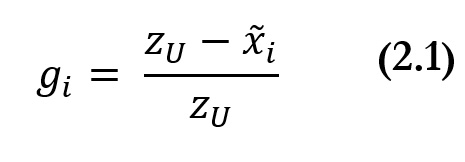 The normalized income gap of person
 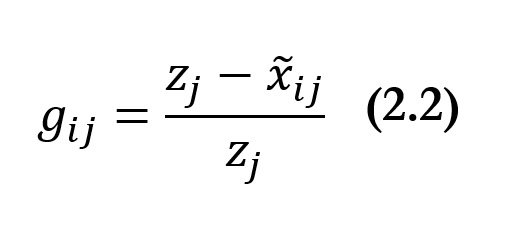 Each
Each 
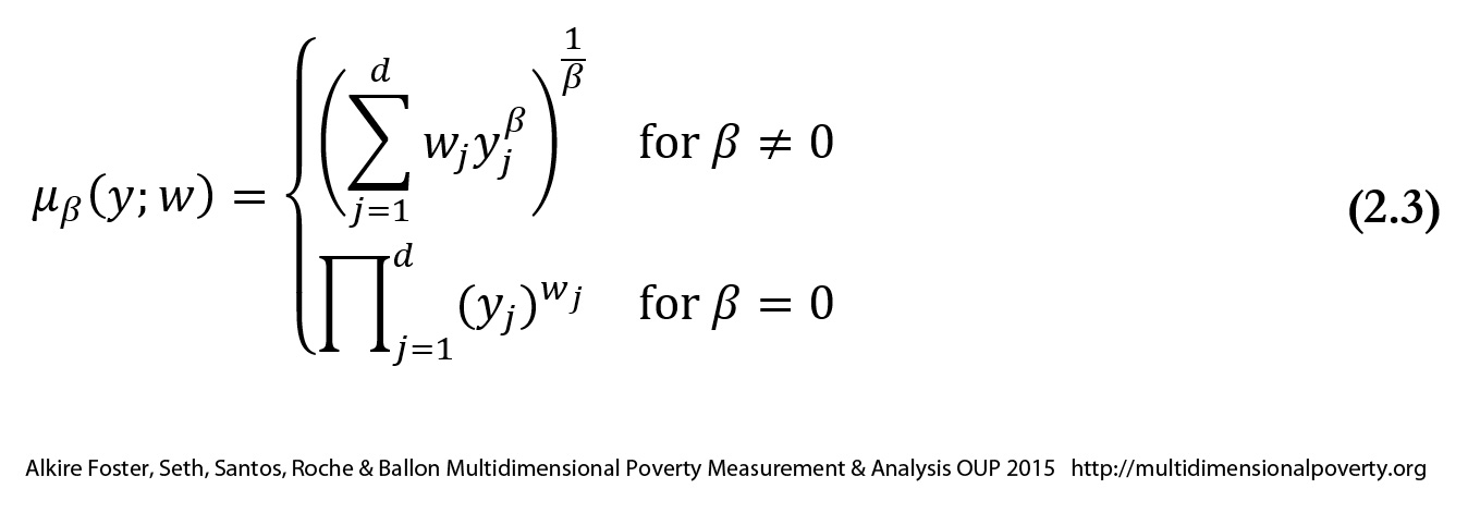 where
where 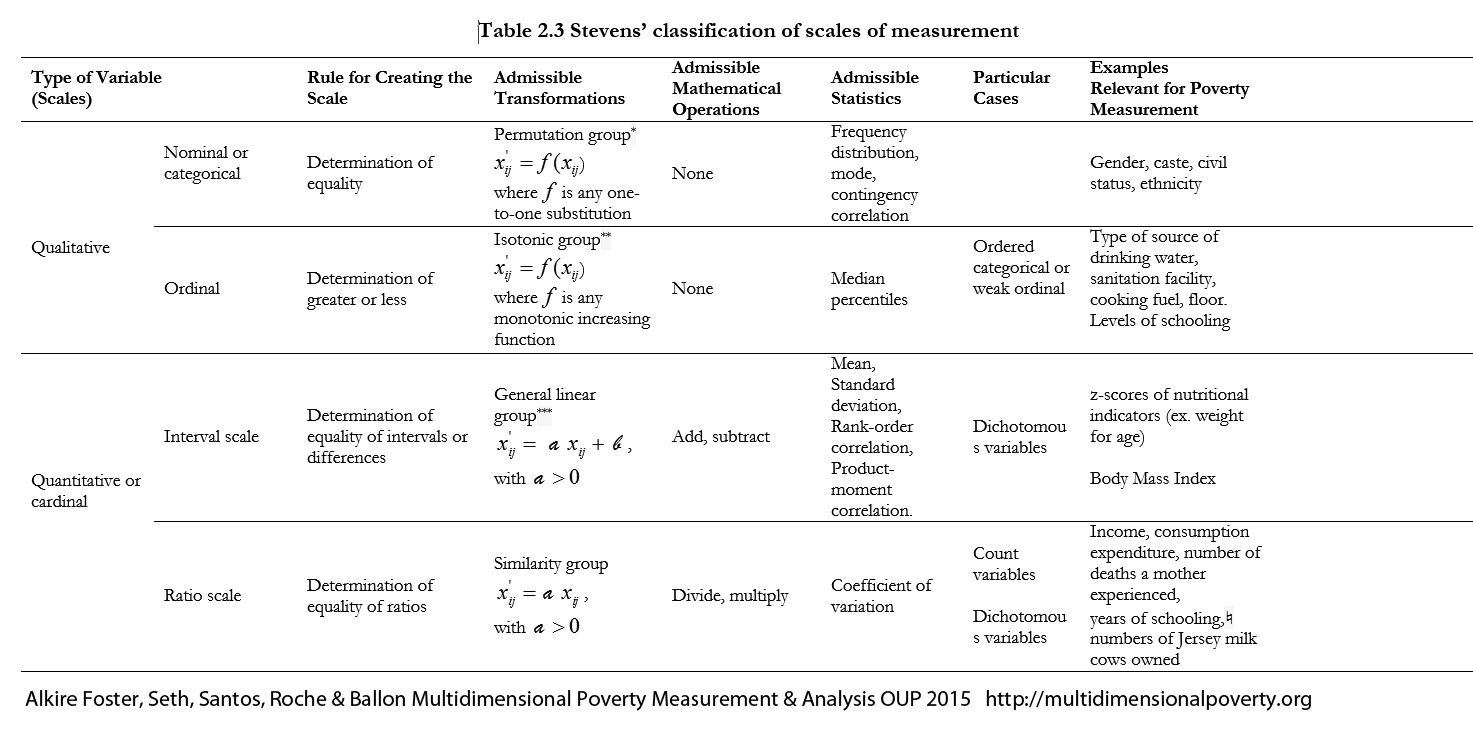
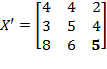 , then by poverty focus,
 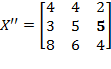 , then by the deprivation focus principle,