
8 Robustness Analysis and Statistical Inference
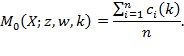
Chapter 5 presented the methodology for the Adjusted Headcount Ratio poverty index ![]() and its different partial indices; Chapter 6 discussed how to design multidimensional poverty measures using this methodology in order to advance poverty reduction; and Chapter 7 explained novel empirical techniques required during implementation. Throughout, we have discussed how the index and its partial indices may be used for policy analysis and decision-making. For example, a central government may want to allocate resources to reduce poverty across its subnational regions or may want to claim credit for strong improvement in the situation of poor people using an implementation of the Adjusted Headcount Ratio. One is, however, entitled to question how conclusive any particular poverty comparisons are for two different reasons.
and its different partial indices; Chapter 6 discussed how to design multidimensional poverty measures using this methodology in order to advance poverty reduction; and Chapter 7 explained novel empirical techniques required during implementation. Throughout, we have discussed how the index and its partial indices may be used for policy analysis and decision-making. For example, a central government may want to allocate resources to reduce poverty across its subnational regions or may want to claim credit for strong improvement in the situation of poor people using an implementation of the Adjusted Headcount Ratio. One is, however, entitled to question how conclusive any particular poverty comparisons are for two different reasons.
One reason is that the design of a poverty measure involves the selection of a set of parameters, and one may ask how sensitive policy prescriptions are to these parameter choices. Any comparison or ranking based on a particular poverty measure may alter when a different set of parameters, such as the poverty cutoff, deprivation cutoffs or weights, is used. We define an ordering as robust with respect to a particular parameter when the order is maintained despite a change in that parameter.[1] The ordering can refer to the poverty ordering of two aggregate entities, say two countries or other geographical entities, which is a pairwise comparison, but it can also refer to the order of more than two entities, what we refer to as a ranking. Clearly, the robustness of a ranking (of several entities) depends on the robustness of all possible pairwise comparisons. Thus, the robustness of poverty comparisons should be assessed for different, but reasonable, specifications of parameters. In many circumstances, the policy-relevant comparisons should be robust to a range of plausible parameter specifications. This process is referred as robustness analysis. There are different ways in which the robustness of an ordering can be assessed. This chapter presents the most widely implemented analyses; new procedures and tests may be developed in the near future.
The second reason for questioning claimed poverty comparisons is that poverty figures in most cases are estimated from sample surveys for drawing inferences about a population. Thus, it is crucial that inferential errors are also estimated and reported. This process of drawing conclusions about the population from the data that are subject to random variation is referred as statistical inference. Inferential errors affect the degree of certainty with which two and more entities may be compared in terms of poverty for a particular set of parameters’ values. Essentially, the difference in poverty levels between two entities – states for example – may or may not be statistically significant. Statistical inference affects not only the poverty comparisons for a particular set of parameter values but also the robustness of such comparisons for a range of parameters’ values.
In general, assessments of robustness should cohere with a measure’s policy use. If the policy depends on levels of ![]() , then the robustness of the respective levels (or ranks) of poverty should be the subject of robustness tests presented here. If the policy uses information on the dimensional composition of poverty, robustness tests should assess these—which lie beyond the scope of this chapter, but see Ura et al. (2012). Recall also from Chapter 6 people’s values may generate plausible ranges of parameters. Robustness tests clarify the extent to which the same policies would be supported across that relevant range of parameters. In this way, robustness tests can be used for building consensus or for clarifying which points of dissensus have important policy implications.
, then the robustness of the respective levels (or ranks) of poverty should be the subject of robustness tests presented here. If the policy uses information on the dimensional composition of poverty, robustness tests should assess these—which lie beyond the scope of this chapter, but see Ura et al. (2012). Recall also from Chapter 6 people’s values may generate plausible ranges of parameters. Robustness tests clarify the extent to which the same policies would be supported across that relevant range of parameters. In this way, robustness tests can be used for building consensus or for clarifying which points of dissensus have important policy implications.
This chapter is divided into two sections. Section 8.1 presents a number of useful tools for conducting different types of robustness analysis; section 8.2 presents various techniques for drawing statistical inferences and section 8.3 presents some ways in which the two types of techniques can be brought together.
8.1 Robustness Analysis
In monetary poverty measures, the parameters include (a) the set of indicators (components of income or consumption); (b) the price vectors used to construct the aggregate as well as any adjustments such as for inflation or urban/rural price differentials; (c) the poverty line; and (d) equivalence scales (if applied). The parameters that influence the multidimensional poverty estimates and poverty comparisons based on the Adjusted Headcount Ratio are (i) the set of indicators (denoted by subscript ![]() ); (ii) the set of deprivation cutoffs (denoted by vector
); (ii) the set of deprivation cutoffs (denoted by vector ![]() ); (iii) the set of weights or deprivation values (denoted by vector
); (iii) the set of weights or deprivation values (denoted by vector ![]() ); and (iv) the poverty cutoff (denoted by
); and (iv) the poverty cutoff (denoted by ![]() ). A change in these parameters may affect the overall poverty estimate or comparisons across regions or countries.
). A change in these parameters may affect the overall poverty estimate or comparisons across regions or countries.
This section introduces tools that can be used to test the robustness of pairwise comparisons as well as the robustness of overall rankings with respect to the initial choice of the parameters. We first introduce a tool to test the robustness of pairwise comparisons with respect to the choice of the poverty cutoff. This tool tests an extreme form of robustness, borrowing from the concept of stochastic dominance in the single-dimensional context (section 3.3.1).[2] When dominance conditions are satisfied, the strongest possible results are obtained. However, as dominance conditions are highly stringent and dominance tests may not hold for a large number of the pairwise comparisons, we present additional tools for assessing the robustness of country rankings using the correlation between different rankings. This second set of tools can be used with changes in any of the other parameters too, namely, weights, indicators and deprivation cutoffs.
8.1.1 Dominance Analysis for Changes in the Poverty Cutoff
Although measurement design begins with the selection of indicators, weights, and deprivation cutoffs, we begin our robustness analysis by assessing dominance with respect to changes in the poverty cutoff, which is applied to the weighted deprivation scores constructed using other parameters. We do this because as in the unidimensional context, it is the poverty cutoff that finally identifies who is poor, thereby defining the ‘headcount ratio’ and effectively setting the level of poverty. It is arguably most visibly debated.[3] We have introduced the concept of stochastic dominance in the uni- and multidimensional context in section 3.3.1. This part of the chapter builds on that concept and technique, focusing primarily on the first-order stochastic dominance (FSD) and showing how it can be applied to identify any unambiguous comparisons with respect to the poverty cutoff for our two most widely used poverty measures—Adjusted Headcount Ratio (![]() ) and Multidimensional Headcount Ratio (
) and Multidimensional Headcount Ratio (![]() ). Recall from section 3.3.1 the notation of two univariate distributions of achievements
). Recall from section 3.3.1 the notation of two univariate distributions of achievements ![]() and
and ![]() with cumulative distribution functions (CDF)
with cumulative distribution functions (CDF) ![]() and
and ![]() , where
, where ![]() and
and ![]() are the shares of population in distributions
are the shares of population in distributions ![]() and
and ![]() with achievement level less than
with achievement level less than ![]() . Distribution
. Distribution ![]() first-order stochastically dominates distribution
first-order stochastically dominates distribution ![]() (or
(or ![]() FSD
FSD ![]() if and only if
if and only if ![]() for all
for all ![]() and
and ![]() for some
for some ![]() . Strict FSD requires that
. Strict FSD requires that ![]() for all
for all ![]() .[4] Interestingly, if distribution
.[4] Interestingly, if distribution ![]() FSD
FSD ![]() , then
, then ![]() has no lower headcount ratio than
has no lower headcount ratio than ![]() for all poverty lines.
for all poverty lines.
Let us now explain how we can apply this concept for unanimous pairwise comparisons using ![]() and
and ![]() between any two distributions of deprivation scores across the population. For a given deprivation cutoff vector
between any two distributions of deprivation scores across the population. For a given deprivation cutoff vector ![]() and a given weighting vector
and a given weighting vector ![]() , the FSD tool can be used to evaluate the sensitivity of any pairwise comparison to varying poverty cutoff
, the FSD tool can be used to evaluate the sensitivity of any pairwise comparison to varying poverty cutoff ![]() . Following the notation introduced in Chapter 2, we denote the (uncensored) deprivation score vector by
. Following the notation introduced in Chapter 2, we denote the (uncensored) deprivation score vector by ![]() . Note that an element of
. Note that an element of ![]() denotes the deprivation score and a larger deprivation score implies a lower level of well-being.
denotes the deprivation score and a larger deprivation score implies a lower level of well-being.
The FSD tool can be applied in two different ways: one is to convert deprivations into attainments by transforming the deprivation score vector ![]() into an attainment score vector 1
into an attainment score vector 1 ![]() and the other option is to use the tool directly on the deprivation score vector
and the other option is to use the tool directly on the deprivation score vector ![]() . The first approach has been pursued in Alkire and Foster (2011a) and Lasso de la Vega (2010). In this section, because it is more direct, we present the results using the deprivation score vector and thus avoid any transformation. A person is identified as poor if the deprivation score is larger than or equal to the poverty cutoff
. The first approach has been pursued in Alkire and Foster (2011a) and Lasso de la Vega (2010). In this section, because it is more direct, we present the results using the deprivation score vector and thus avoid any transformation. A person is identified as poor if the deprivation score is larger than or equal to the poverty cutoff ![]() , unlike in the attainment space where a person is identified as poor if the person’s attainment falls below a certain poverty cutoff. To do that, however, we need to introduce the complementary cumulative distribution function (CCDF)—the complement of a CDF.[5] For any distribution
, unlike in the attainment space where a person is identified as poor if the person’s attainment falls below a certain poverty cutoff. To do that, however, we need to introduce the complementary cumulative distribution function (CCDF)—the complement of a CDF.[5] For any distribution ![]() with CDF
with CDF ![]() , the CCDF of the distribution is
, the CCDF of the distribution is ![]() 1
1 ![]() , which means that for any value
, which means that for any value ![]() , the CCDF
, the CCDF ![]() is the proportion of the population that has values larger than or equal to
is the proportion of the population that has values larger than or equal to ![]() . Naturally, CCDFs are downward sloping. The first-order stochastic dominance condition in terms of the CCDFs can be stated as follows. Any distribution
. Naturally, CCDFs are downward sloping. The first-order stochastic dominance condition in terms of the CCDFs can be stated as follows. Any distribution ![]() first order stochastically dominates distribution
first order stochastically dominates distribution ![]() if and only if
if and only if ![]() for all
for all ![]() and
and ![]() for some
for some ![]() . For strict FSD, the strict inequality must hold for all
. For strict FSD, the strict inequality must hold for all ![]() .
.
Now, suppose there are two distributions of deprivation scores, ![]() and
and ![]() with CCDFs
with CCDFs ![]() and
and ![]() . For poverty cutoff
. For poverty cutoff ![]() , if
, if ![]() , then distribution
, then distribution ![]() has no lower multidimensional headcount ratio
has no lower multidimensional headcount ratio ![]() than distribution
than distribution ![]() at
at ![]() . When is it possible to say that distribution
. When is it possible to say that distribution ![]() has no lower
has no lower ![]() than distribution
than distribution ![]() for all poverty cutoffs? The answer is when distribution
for all poverty cutoffs? The answer is when distribution ![]() first order stochastically dominates distribution
first order stochastically dominates distribution ![]() . Let us provide an example in terms of two four-person vectors of deprivation scores:
. Let us provide an example in terms of two four-person vectors of deprivation scores: ![]() and
and ![]() . The corresponding CCDFs
. The corresponding CCDFs ![]() and
and ![]() are denoted by a black dotted line and a solid grey line, respectively, in Figure 8.1. No part of
are denoted by a black dotted line and a solid grey line, respectively, in Figure 8.1. No part of ![]() lies above that of
lies above that of ![]() and so
and so ![]() first-order stochastically dominates
first-order stochastically dominates ![]() and we can conclude that
and we can conclude that ![]() has unambiguously lower poverty than
has unambiguously lower poverty than ![]() , in terms of the multidimensional headcount ratio.
, in terms of the multidimensional headcount ratio.
Figure 8.1 Complementary CDFs and Poverty Dominance
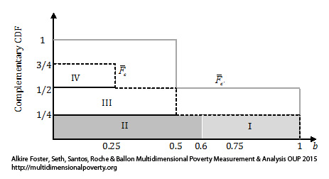
Let us now try to understand dominance in terms of ![]() . In order to do so, first note that the area underneath a CCDF of a deprivation score vector is the average of its deprivation scores. Consider distribution
. In order to do so, first note that the area underneath a CCDF of a deprivation score vector is the average of its deprivation scores. Consider distribution ![]() with CCDF
with CCDF ![]() as in Figure 8.1. The area underneath
as in Figure 8.1. The area underneath ![]() is the sum of areas I, II, III, and IV. Area IV is equal to
is the sum of areas I, II, III, and IV. Area IV is equal to ![]() , Area III is
, Area III is ![]() , and Areas I+II is
, and Areas I+II is ![]() , so essentially each area is a score times its frequency in the population. The sum of the four areas
, so essentially each area is a score times its frequency in the population. The sum of the four areas ![]() , is simply the average of all elements in
, is simply the average of all elements in ![]() and it coincides with the
and it coincides with the ![]() measure for a union approach. When an intermediate or intersection approach to identification is used, then the
measure for a union approach. When an intermediate or intersection approach to identification is used, then the ![]() is the average of the censored deprivation score vector
is the average of the censored deprivation score vector ![]() . In other words, the deprivation scores of those who are not identified as poor are set to 0. For example, for a poverty cutoff
. In other words, the deprivation scores of those who are not identified as poor are set to 0. For example, for a poverty cutoff ![]() , the censored deprivation score vector corresponding to
, the censored deprivation score vector corresponding to ![]() is
is ![]() . Obtaining the average of censored deprivation scores is equivalent to ignoring areas III and IV in Figure 8.1. The
. Obtaining the average of censored deprivation scores is equivalent to ignoring areas III and IV in Figure 8.1. The ![]() of
of ![]() for
for ![]() is the sum of the remaining area I, II which is
is the sum of the remaining area I, II which is ![]() .[6]
.[6]
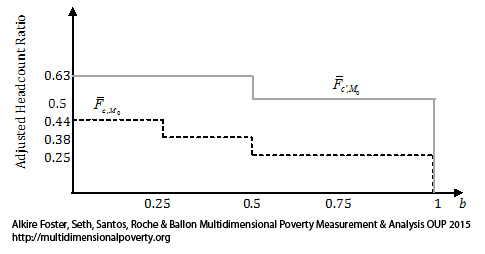
We now compute the area underneath the censored CCDF for every ![]() and plot the area on the vertical axis for each
and plot the area on the vertical axis for each ![]() on the horizontal axis and refer to it as an
on the horizontal axis and refer to it as an ![]() curve, depicted in Figure 8.2. We denote the
curve, depicted in Figure 8.2. We denote the ![]() curves of distributions
curves of distributions ![]() and
and ![]() by
by ![]() and
and ![]() , respectively. Given that the
, respectively. Given that the ![]() curves are obtained by computing the areas underneath the CCDFs, the dominance of
curves are obtained by computing the areas underneath the CCDFs, the dominance of ![]() curves is referred as second-order stochastic dominance. Given that first-order stochastic dominance implies second-order dominance, if first-order dominance holds between two distributions, then
curves is referred as second-order stochastic dominance. Given that first-order stochastic dominance implies second-order dominance, if first-order dominance holds between two distributions, then ![]() dominance will also hold between them. However, the converse is not necessarily true, that is, even when there is
dominance will also hold between them. However, the converse is not necessarily true, that is, even when there is ![]() dominance there may not be
dominance there may not be ![]() dominance. Therefore, when the CCDFs of two distributions cross—i.e. there is not first-order (
dominance. Therefore, when the CCDFs of two distributions cross—i.e. there is not first-order (![]() ) dominance—it is worth testing
) dominance—it is worth testing ![]() dominance between pairs of distributions, to which we refer as pairwise comparisons from now on, using the
dominance between pairs of distributions, to which we refer as pairwise comparisons from now on, using the ![]() curves. Batana (2013) has used the
curves. Batana (2013) has used the ![]() curves for the purpose of robustness analysis while comparing multidimensional poverty among women in fourteen African countries.
curves for the purpose of robustness analysis while comparing multidimensional poverty among women in fourteen African countries.
Figure 8.2 The Adjusted Headcount Ratio Dominance Curves
The dominance requirement for all possible poverty cutoffs may be an excessively stringent requirement. Practically, one may seek to verify the unambiguity of comparison with respect to a limited variation the poverty cutoff, which can be referred to as restricted dominance analysis. For example, when making international comparisons in terms of the MPI, Alkire and Santos (2010, 2014) tested the robustness of pairwise comparisons for all poverty cutoffs ![]() [0.2, 0.4], in addition to the poverty cutoff of
[0.2, 0.4], in addition to the poverty cutoff of ![]() 1/3. In this case, if the restricted FSD holds between any two distributions, then dominance holds for the relevant particular range of poverty cutoffs for both
1/3. In this case, if the restricted FSD holds between any two distributions, then dominance holds for the relevant particular range of poverty cutoffs for both ![]() and
and ![]() .
.
8.1.2 Rank Robustness Analysis
In situations in which dominance tests are too stringent, we may explore a milder form of robustness, which assesses the extent to which a ranking, that is, an ordering of more than two entities, obtained under a specific set of parameters’ values, is preserved when the value of some parameter is modified. How should we assess the robustness of a ranking? One first intuitive measure is to compute the percentage of pairwise comparisons that are robust to changes in parameters – that is the proportion of pairwise comparisons that have the same ordering. As we shall see in section 8.3, whenever poverty computations are performed using a survey, the statistical inference tools need to be incorporated into the robustness analysis.
Another useful way to assess the robustness of a ranking is by computing a rank correlation coefficient between the original ranking of entities and the alternative rankings (i.e. those obtained with alternative parameters’ values). There are various choices for a rank correlation coefficient. The two most commonly used rank correlation coefficients are the Spearman rank correlation coefficient (![]() ) and the Kendall rank correlation coefficient (
) and the Kendall rank correlation coefficient (![]() ).[7]
).[7]
Suppose, for a particular parametric specification, the set of ranks across ![]() population subgroups is denoted by
population subgroups is denoted by ![]() , where
, where ![]() is the rank attributed to subgroup
is the rank attributed to subgroup ![]() . The subgroups may be ranked by their level of multidimensional headcount ratio, the Adjusted Headcount Ratio, or any other partial indices. We present the rank correlation measures using population subgroups, but they apply to ranking across countries as well. We denote the set of ranks for an alternative specification of parameters by
. The subgroups may be ranked by their level of multidimensional headcount ratio, the Adjusted Headcount Ratio, or any other partial indices. We present the rank correlation measures using population subgroups, but they apply to ranking across countries as well. We denote the set of ranks for an alternative specification of parameters by ![]() , where
, where ![]() is the rank attributed to subgroup
is the rank attributed to subgroup ![]() . The alternative specification may be a different poverty cutoff, a different set of deprivation cutoffs, a different set of weights, or a combination of all three. If the initial and the alternative specification yield exactly the same set of rankings across subgroups, then
. The alternative specification may be a different poverty cutoff, a different set of deprivation cutoffs, a different set of weights, or a combination of all three. If the initial and the alternative specification yield exactly the same set of rankings across subgroups, then ![]() for all
for all ![]() . In this case, we state that the two sets of rankings are perfectly positively associated and the association is highest across the two specifications. In terms of the previous approach, 100% of the pairwise comparisons are robust to changes in one or more parameters’ values. On the other hand, if the two specifications yield completely opposite sets of rankings, then
. In this case, we state that the two sets of rankings are perfectly positively associated and the association is highest across the two specifications. In terms of the previous approach, 100% of the pairwise comparisons are robust to changes in one or more parameters’ values. On the other hand, if the two specifications yield completely opposite sets of rankings, then ![]() for all
for all ![]() . In this case, we state that the two sets of rankings are perfectly negatively associated and the association is lowest across the two specifications. In terms of the previous approach, 0% of the pairwise comparisons are robust to changes in one or more parameters’ values.
. In this case, we state that the two sets of rankings are perfectly negatively associated and the association is lowest across the two specifications. In terms of the previous approach, 0% of the pairwise comparisons are robust to changes in one or more parameters’ values.
The Spearman rank correlation coefficient can be expressed as
|
|
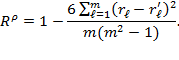
Intuitively, for the Spearman rank correlation coefficient, the square of the difference in the two ranks for each subgroup is computed and an average is taken across all subgroups. The ![]() is bounded between
is bounded between ![]() and
and ![]() . The lowest value of
. The lowest value of ![]() is obtained when two rankings are perfectly negatively associated with each other whereas the largest value of
is obtained when two rankings are perfectly negatively associated with each other whereas the largest value of ![]() is obtained when two rankings are perfectly positively associated with each other.
is obtained when two rankings are perfectly positively associated with each other.
The Kendall rank correlation coefficient is based on the number of concordant pairs and discordant pairs. A pair (![]() ) is concordant if the comparisons between two objects are the same in both the initial and alternative specification, i.e.
) is concordant if the comparisons between two objects are the same in both the initial and alternative specification, i.e. ![]() and
and ![]() . In terms of the previously used terms, a concordant pair is equivalent to a robust pairwise comparison. A pair, on the other hand, is discordant if the comparisons between two objects are altered between the initial and the alternative specification such that
. In terms of the previously used terms, a concordant pair is equivalent to a robust pairwise comparison. A pair, on the other hand, is discordant if the comparisons between two objects are altered between the initial and the alternative specification such that ![]() but
but ![]() . In terms of the previously used terms, a discordant pair is equivalent to a non-robust pairwise comparison. The
. In terms of the previously used terms, a discordant pair is equivalent to a non-robust pairwise comparison. The ![]() is the difference in the number of concordant and discordant pairs divided by the total number of pairwise comparisons. The Kendall rank correlation coefficient can be expressed as
is the difference in the number of concordant and discordant pairs divided by the total number of pairwise comparisons. The Kendall rank correlation coefficient can be expressed as
|
|
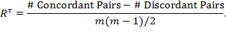
Like ![]() ,
, ![]() also lies between
also lies between ![]() and
and ![]() . The lowest value of
. The lowest value of ![]() is obtained when two rankings are perfectly negatively associated with each other whereas the largest value of
is obtained when two rankings are perfectly negatively associated with each other whereas the largest value of ![]() is obtained when two rankings are perfectly positively associated with each other. Although both
is obtained when two rankings are perfectly positively associated with each other. Although both ![]() and
and ![]() are used to assess rank robustness the Kendall rank correlation coefficient has an intuitive interpretation. Suppose the Kendall Tau correlation coefficient is 0.90, from equation (8.2), it can be deduced that this means that 95% of the pairwise comparisons are concordant (i.e. robust) and only 5% are discordant. Equations (8.1) and (8.2) are based on the assumption that there are no ties in the rankings. In other words, both expressions are applicable when no two entities have equal values. When there are ties, Kendall (1970) offers two adjustments in the denominator of both rank correlation coefficients (
are used to assess rank robustness the Kendall rank correlation coefficient has an intuitive interpretation. Suppose the Kendall Tau correlation coefficient is 0.90, from equation (8.2), it can be deduced that this means that 95% of the pairwise comparisons are concordant (i.e. robust) and only 5% are discordant. Equations (8.1) and (8.2) are based on the assumption that there are no ties in the rankings. In other words, both expressions are applicable when no two entities have equal values. When there are ties, Kendall (1970) offers two adjustments in the denominator of both rank correlation coefficients (![]() and
and ![]() ) to correct for tied ranks; these adjusted Kendall coefficients are commonly known as tau-b and tau-c.
) to correct for tied ranks; these adjusted Kendall coefficients are commonly known as tau-b and tau-c.
Table 8.1 Correlation among Country Ranks for Different Weights[8]

Let us present one empirical illustration showing how rank robustness tools may be used in practice. The first illustration presents the correlation between 2011 MPI rankings across 109 countries and the rankings for three alternative weighting vectors (Alkire et al. 2011). The MPI attaches equal weights across three dimensions: health, education, and standard of living. However, it is hard to argue with perfect confidence that the initial weight is the correct choice. Therefore, three alternative weighting schemes were considered. The first alternative assigns a 50% weight to the health dimension and then a 25% weight to each of the other two dimensions. Similarly, the second alternative assigns a 50% weight to the education dimension and then distributes the rest of the weight equally across the other two dimensions. The third alternative specification attaches a 50% weight to the standard of living dimension and then 25% weights to each of the other two dimensions. Thus, we now have four different rankings of 109 countries, each involving 5,356 pairwise comparisons. Table 8.1 presents the rank correlation coefficient ![]() and
and ![]() between the initial ranking and the ranking for each alternative specification. It can be seen that the Spearman coefficient is around 0.98 for all three alternatives. The Kendall coefficient is around 0.9 for each of the three cases, implying that around 80% of the comparisons are concordant in each case.
between the initial ranking and the ranking for each alternative specification. It can be seen that the Spearman coefficient is around 0.98 for all three alternatives. The Kendall coefficient is around 0.9 for each of the three cases, implying that around 80% of the comparisons are concordant in each case.
The same type of analysis has been done to changes in other parameters’ values, such as the indicators used and deprivation cutoffs (Alkire and Santos 2014).
8.2 Statistical Inference
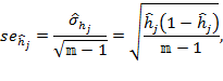
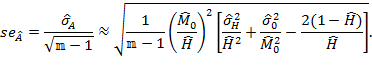
The last section showed how the robustness of claims made using the Adjusted Headcount Ratio and its partial indices may be assessed. Such assessments apply to changes in a country’s performance over time, comparisons between different countries, and comparisons of different population subgroups within a country. Most frequently, the indices are estimated from sample surveys with the objective of estimating the unknown population parameters as accurately as possible. A sample survey, unlike a census that covers the entire population, consists of a representative fraction of the population.[9] Different sample surveys, even when conducted at the same time and despite having the same design, would most likely provide a different set of estimates for the same population parameters. Thus, it is crucial to compute a measure of confidence or reliability for each estimate from a sample survey. This is done by computing the standard deviation of an estimate. The standard deviation of an estimate is referred to as its standard error. The lower the magnitude of a standard error, the larger the reliability of the corresponding estimate. Standard errors are key for hypothesis testing and for the construction of confidence intervals, both of which are very helpful for robustness analysis and more generally for drawing policy conclusions. In what follows we briefly explain each of these statistical terms.
8.2.1 Standard Errors
There are different approaches to estimating standard errors. Two approaches are commonly followed:
- Analytical Approach: Formulas that provide either the exact or the asymptotic approximation of the standard error and thus confidence intervals[10]
- Resampling Approach: Standard errors and the confidence intervals may be computed through the bootstrap or similar techniques (as performed for the global MPI in Alkire and Santos 2014).
The Appendix to this chapter presents the formulas for computing standard errors with the analytical approach depending on the survey design.
The analytical approach is based on two assumptions. Such assumptions are based on the premise that the sample surveys used for estimating the population parameters are significantly smaller in size compared to the population size under consideration.[11] For example, the sample size of the Demographic and Health Survey of India in 2006 was only 0.04% of the Indian population. The first assumption is that the samples are drawn from a population that is infinitely large, so that even the finite population under study is a sample of an infinitely large superpopulation. This philosophical assumption is based on the superpopulation approach, which is different from the finite population approach (for further discussion see Deaton 1997). A finite population approach requires that a finite population correction factor should be used to deflate the standard error if the sample size is large relative to the population. However, if the sample size is significantly smaller than the finite population size, the finite population correction factor is approximately equal to one. In this case, the standard errors based on both approaches are almost the same.
The second assumption is that we treat each sample as drawn from the population with replacement. The practical motivation behind the assumption is the size of the sample survey compared to the population. The sample surveys are commonly conducted without replacement because, once a household is visited and interviewed, the same household is not visited again on purpose. When samples are drawn with replacement, the observations are independent of each other. However, if the samples are drawn without replacement, then the samples are not independent of each other. It can be shown that in the absence of multistage sampling, a sampling without replacements needs a Finite Population Correction (FPC) factor for computing the sampling variance. The FPC factor is of the order ![]() , where
, where ![]() is the sample size and
is the sample size and ![]() is the size of the population. The use of an FPC factor allows us to get a better estimate of the true population variance. However, when the sample size is small with respect to the population, i.e.
is the size of the population. The use of an FPC factor allows us to get a better estimate of the true population variance. However, when the sample size is small with respect to the population, i.e. ![]() , the use of an FPC factor will not make much difference to the estimation of the sampling variance as the FPC factor is closer to one (Duclos and Araar 2006: 276). These assumptions would be required in order to justify our assumption that each sample is independently and identically distributed.
, the use of an FPC factor will not make much difference to the estimation of the sampling variance as the FPC factor is closer to one (Duclos and Araar 2006: 276). These assumptions would be required in order to justify our assumption that each sample is independently and identically distributed.
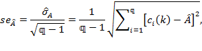
We now illustrate relevant methods using the Adjusted Headcount Ratio (![]() ) denoting its sample estimate by
) denoting its sample estimate by ![]() and standard error of the estimate by
and standard error of the estimate by ![]() . However, the methods are equally applicable to inferences for the multidimensional headcount ratio, the intensity, and the censored headcount ratios as long the standard errors are appropriately computed, as outlined in the Appendix of this chapter.
. However, the methods are equally applicable to inferences for the multidimensional headcount ratio, the intensity, and the censored headcount ratios as long the standard errors are appropriately computed, as outlined in the Appendix of this chapter.
8.2.2 Confidence Intervals
A confidence interval of a point estimate is an interval that contains the true population parameter with some probability that is known as its confidence level. A significance level that is used is the complement of the confidence level. Let us denote the significance level[12] by ![]() , which by definition ranges between 0 and 100%. The level of confidence is
, which by definition ranges between 0 and 100%. The level of confidence is ![]() percent. Thus, for a given estimate, if one wants to be 95% confident about the range within which the true population parameter lies, then the significance is 5%. Similarly, if one wants to be 99% confident, then the significance level is 1%.
percent. Thus, for a given estimate, if one wants to be 95% confident about the range within which the true population parameter lies, then the significance is 5%. Similarly, if one wants to be 99% confident, then the significance level is 1%.
By the central limit theorem, we can say that the difference between the population parameter and the corresponding sample average divided by the standard error approximates the standard normal distribution (i.e. the normal distribution with a mean of 0 and a standard deviation of 1). Using the standard normal distribution one can determine the critical value associated with that significance level, which is given by the inverse of the standard normal distribution at ![]() . In other words, the critical value is the value at which the probability that the statistic is higher than that is precisely
. In other words, the critical value is the value at which the probability that the statistic is higher than that is precisely ![]() .[13] The critical values to be used when one is interested in computing a 95% confidence interval are:
.[13] The critical values to be used when one is interested in computing a 95% confidence interval are: ![]() . If instead one is interested in computing a 99% or a 90% confidence interval, the corresponding critical values are
. If instead one is interested in computing a 99% or a 90% confidence interval, the corresponding critical values are ![]() and
and ![]() , respectively.
, respectively.
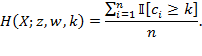
For example, Table 8.2 presents the sample estimate of the Adjusted Headcount Ratio (![]() ), the multidimensional headcount ratio (
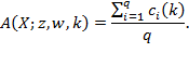
), the multidimensional headcount ratio (![]() ), and the average deprivation share among the poor (
), and the average deprivation share among the poor (![]() ) from the Demographic and Health Survey of 2005–2006. India’s sample estimate of the population-Adjusted Headcount Ratio is
) from the Demographic and Health Survey of 2005–2006. India’s sample estimate of the population-Adjusted Headcount Ratio is ![]() , with a standard error
, with a standard error ![]() . The
. The ![]() % confidence interval is then
% confidence interval is then ![]() . This means that with 95% confidence, the true population
. This means that with 95% confidence, the true population ![]() lies between
lies between ![]() and
and ![]() . Similarly, the 99% confidence interval of India’s
. Similarly, the 99% confidence interval of India’s ![]() is (
is (![]() ). The more one wants to be confident about the range within which the true population parameter lies, the larger the confidence interval will be.
). The more one wants to be confident about the range within which the true population parameter lies, the larger the confidence interval will be.
Confidence Intervals for ![]() ,
, ![]() , and
, and ![]()
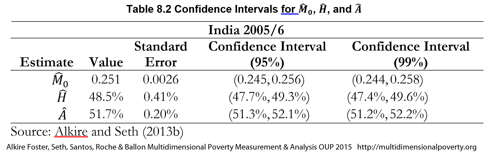
Similar to ![]() , the confidence interval for
, the confidence interval for ![]() is
is ![]() , for
, for ![]() is
is ![]() , and for
, and for ![]() is
is ![]() for all
for all ![]() . It can be seen from the table that the standard error of
. It can be seen from the table that the standard error of ![]() is 0.41%, whereas that of
is 0.41%, whereas that of ![]() is 0.20%.
is 0.20%.
8.2.3 Hypothesis Tests
Confidence intervals are useful for judging the statistical reliability of a point estimate when the population parameter is unknown. However, suppose that, somehow, we have a hypothesis about what the population parameter is. For example, suppose the government hypothesizes that the Adjusted Headcount Ratio in India is 0.26. Thus, the null hypothesis is ![]() . This has to be tested against any of the three alternatives
. This has to be tested against any of the three alternatives ![]() or
or ![]() or
or ![]() .[14] This is a one-sample test. Note that the first alternative requires a so-called two-tailed test, and each of the other two alternatives requires a so-called one-tailed test. Now, suppose a sample (either simple random or multistage stratified)
.[14] This is a one-sample test. Note that the first alternative requires a so-called two-tailed test, and each of the other two alternatives requires a so-called one-tailed test. Now, suppose a sample (either simple random or multistage stratified) ![]() of size
of size ![]() is collected. We denote the estimated Adjusted Headcount Ratio by
is collected. We denote the estimated Adjusted Headcount Ratio by ![]() . By the law of large numbers and by the central limit theorem, as
. By the law of large numbers and by the central limit theorem, as ![]() ,
, ![]() , where
, where ![]() is the population variance of
is the population variance of ![]() . The standard error
. The standard error ![]() of
of ![]() can be estimated using either equation (8.11) or (8.30) in the Appendix, whichever is applicable.
can be estimated using either equation (8.11) or (8.30) in the Appendix, whichever is applicable.
In a two-tail test, the null hypothesis can be rejected against the alternative ![]() with (
with (![]() ) percent confidence if
) percent confidence if ![]() .; in words, if the absolute value of the statistic is greater than the absolute value of the critical value. An equivalent procedure to reject or not the null hypothesis entails, rather than comparing the test statistic against the critical value, comparing the significance level against the so-called
.; in words, if the absolute value of the statistic is greater than the absolute value of the critical value. An equivalent procedure to reject or not the null hypothesis entails, rather than comparing the test statistic against the critical value, comparing the significance level against the so-called ![]() -value. The
-value. The ![]() -value is defined as the actual probability that the test statistic assumes a value greater than the value observed, i.e. it is the probability of rejecting the null hypothesis when it is true.
-value is defined as the actual probability that the test statistic assumes a value greater than the value observed, i.e. it is the probability of rejecting the null hypothesis when it is true.
Let us consider the example of India’s Adjusted Headcount Ratio, reported in Table 8.2, where ![]() and
and ![]() . Now,
. Now, ![]() . Thus, with
. Thus, with ![]() % confidence, the null hypothesis can be rejected with respect to the alternative
% confidence, the null hypothesis can be rejected with respect to the alternative ![]() and the corresponding
and the corresponding ![]() -value is
-value is ![]() , where
, where ![]() stands for the cumulative standard normal distribution. Similarly, in a one-tail test to the right, the null hypothesis can be rejected against the alternative
stands for the cumulative standard normal distribution. Similarly, in a one-tail test to the right, the null hypothesis can be rejected against the alternative ![]() with (
with (![]() ) percent confidence if
) percent confidence if ![]() . The corresponding
. The corresponding ![]() -value is
-value is ![]() . Finally, in a one tail test to the left, the null hypothesis can be rejected against the alternative
. Finally, in a one tail test to the left, the null hypothesis can be rejected against the alternative ![]() with (
with (![]() ) percent confidence, if
) percent confidence, if ![]() , where the relevant
, where the relevant ![]() -value is
-value is ![]() .[15]
.[15]
Note that the conclusions based on the confidence intervals and the one-sample tests are identical. If the value at the null hypothesis lies outside of the confidence interval, then the test will also show that null hypothesis is rejected. On the other hand, if the value at the null hypothesis lies inside the confidence interval, then the test cannot reject the null hypothesis.
Formal tests are also required in order to understand whether a change in the estimate over time—or a difference between the estimates of two countries—has been statistically significant. The difference is that this is a two-sample test. We assume that the two estimates whose difference is of interest are estimated from two independent samples.[16] For example, when we are interested in testing the difference in ![]() across two countries, across rural and urban areas, or across population subgroups, it is safe to assume that the samples are drawn independently. A somewhat different situation may arise with a change over time. It is possible that the samples are drawn independently of each other or that the samples are drawn from the same population in order to track changes over time, as, for example, in panel datasets. This section restricts its attention to assessments in which we can assume independent samples.
across two countries, across rural and urban areas, or across population subgroups, it is safe to assume that the samples are drawn independently. A somewhat different situation may arise with a change over time. It is possible that the samples are drawn independently of each other or that the samples are drawn from the same population in order to track changes over time, as, for example, in panel datasets. This section restricts its attention to assessments in which we can assume independent samples.
Suppose there are two countries, Country I and Country II. The population achievement matrices are denoted by ![]() and
and ![]() respectively, and the population Adjusted Headcount Ratios are denoted by
respectively, and the population Adjusted Headcount Ratios are denoted by ![]() and
and ![]() , respectively. We seek to test the null hypothesis
, respectively. We seek to test the null hypothesis ![]() , which implies that poverty in country I is not significantly different from poverty in country II in any of the three alternatives:
, which implies that poverty in country I is not significantly different from poverty in country II in any of the three alternatives: ![]() which means that one of the two countries is significantly poorer than the other; or
which means that one of the two countries is significantly poorer than the other; or ![]() , which means that country I is significantly poorer than country II; or
, which means that country I is significantly poorer than country II; or ![]() , which means the opposite. For the first alternative, we need to conduct a two-tailed test, and for the other two alternatives, we need to conduct a one-tailed test.
, which means the opposite. For the first alternative, we need to conduct a two-tailed test, and for the other two alternatives, we need to conduct a one-tailed test.
Now, suppose a sample (either simple random or multistage stratified) ![]() of size
of size ![]() is collected from
is collected from ![]() and a sample
and a sample ![]() of size
of size ![]() is collected from
is collected from ![]() , where samples in
, where samples in ![]() and
and ![]() are assumed to have been drawn independently of each other. We denote the estimated Adjusted Headcount Ratios from the samples by
are assumed to have been drawn independently of each other. We denote the estimated Adjusted Headcount Ratios from the samples by ![]() and
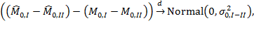
and ![]() , respectively. By the law of large numbers and the central limit theorem,
, respectively. By the law of large numbers and the central limit theorem, ![]() and
and ![]() . The difference of two normal distributions is a normal distribution as well. Thus,
. The difference of two normal distributions is a normal distribution as well. Thus,
|
|
(8.3) |
where 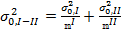 . Note that, as we have assumed independent samples, the covariance between the two Adjusted Headcount Ratios is zero. Hence, the standard error of
 ![]() , denoted by
, denoted by ![]() , may be estimated using equations (8.11) or (8.30) in the Appendix, whichever is applicable, as:
, may be estimated using equations (8.11) or (8.30) in the Appendix, whichever is applicable, as:
|
|
(8.4) |
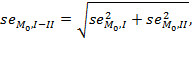
where ![]() is the standard error of
is the standard error of ![]() and
and ![]() is the standard error of
is the standard error of ![]() . Like the one-sample test discussed above, in the two-tail test, the null hypothesis can be rejected against the alternative
. Like the one-sample test discussed above, in the two-tail test, the null hypothesis can be rejected against the alternative ![]() with (
with (![]() ) percent confidence, if
) percent confidence, if ![]() . Given that at the null hypothesis
. Given that at the null hypothesis ![]() , this implies requiring
, this implies requiring ![]() . Similarly, in order to reject the null hypothesis against
. Similarly, in order to reject the null hypothesis against ![]() , we require
, we require ![]() and against
and against ![]() , we require
, we require ![]() The corresponding
The corresponding ![]() -values can be computed as discussed in the one-sample test.
-values can be computed as discussed in the one-sample test.
Table 8.3 presents an example of an estimation of MPI (an adaptation of ![]() ) in four Indian states: Goa, Punjab, Andhra Pradesh, and Tripura, with their corresponding standard errors, confidence intervals and hypothesis tests.[17] These results are computed from the Demographic and Health Survey of India for the years 2005–2006. In the table we can see that the MPI point estimate for Goa is 0.057, and with 95% confidence, we can say that the MPI estimate of Goa lies somewhere between 0.045 and 0.069. Similarly, we can say with 95% confidence that Punjab’s MPI is not larger than 0.103 and no less than 0.073, although the point estimate of MPI is 0.088. We can also state, after doing the corresponding hypothesis test, that Punjab is significantly poorer than Goa. However, we cannot draw the same kind of conclusion for the comparison between Andhra Pradesh and Tripura, although the difference between the MPI estimates of these two states (0.032) is similar to the difference between Goa and Punjab.
) in four Indian states: Goa, Punjab, Andhra Pradesh, and Tripura, with their corresponding standard errors, confidence intervals and hypothesis tests.[17] These results are computed from the Demographic and Health Survey of India for the years 2005–2006. In the table we can see that the MPI point estimate for Goa is 0.057, and with 95% confidence, we can say that the MPI estimate of Goa lies somewhere between 0.045 and 0.069. Similarly, we can say with 95% confidence that Punjab’s MPI is not larger than 0.103 and no less than 0.073, although the point estimate of MPI is 0.088. We can also state, after doing the corresponding hypothesis test, that Punjab is significantly poorer than Goa. However, we cannot draw the same kind of conclusion for the comparison between Andhra Pradesh and Tripura, although the difference between the MPI estimates of these two states (0.032) is similar to the difference between Goa and Punjab.
Table 8.3 Comparison of Indian States Using Standard Errors
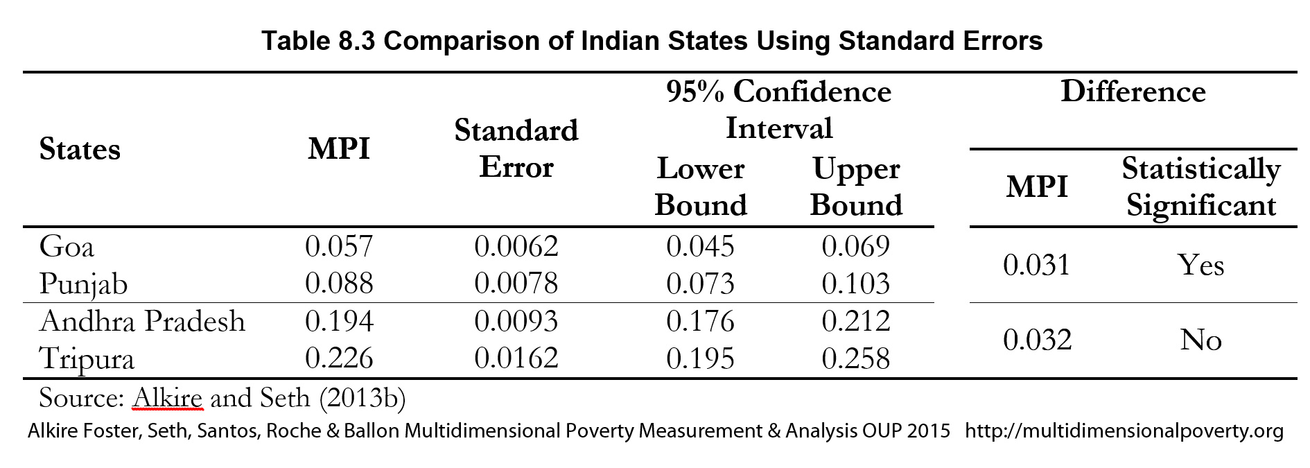
It is vital to understand that in two sample tests, conclusions about the statistical significance obtained with confidence intervals do not necessarily coincide with conclusions obtained using hypothesis testing. Let us formally examine the situation. Suppose, ![]() . If the confidence intervals do not overlap, then the lower bound of
. If the confidence intervals do not overlap, then the lower bound of ![]() is larger than the upper bound of
is larger than the upper bound of ![]() , i.e.
, i.e. ![]() or
or ![]() . Given that for two independent samples,
. Given that for two independent samples, ![]() , if the confidence intervals do not cross, a statistically significant comparison can be made. However, if the confidence intervals overlap, it does not necessarily mean that the comparison is not statistically significant at the same level of significance. It is thus essential to conduct statistical tests on differences when the confidence intervals overlap.
, if the confidence intervals do not cross, a statistically significant comparison can be made. However, if the confidence intervals overlap, it does not necessarily mean that the comparison is not statistically significant at the same level of significance. It is thus essential to conduct statistical tests on differences when the confidence intervals overlap.
8.3 Robustness Analysis with Statistical Inference
In practice, the robustness analyses discussed in section 8.1 are typically performed with estimates from sample surveys. In at least two cases, it is necessary to combine the robustness analyses with the statistical inference tools just described. This section describes how to do so in practice.
The dominance analysis presented in section 8.1.1 assesses dominance between two CCDFs or two ![]() curves in order to conclude whether a pairwise ordering is robust to the choice of all poverty cutoffs. But it is also crucial to examine if the pairwise dominance of the CCDFs or
curves in order to conclude whether a pairwise ordering is robust to the choice of all poverty cutoffs. But it is also crucial to examine if the pairwise dominance of the CCDFs or ![]() curves are statistically significant. For two entities in a pairwise ordering, one should perform one-tailed hypothesis tests of the difference in the two
curves are statistically significant. For two entities in a pairwise ordering, one should perform one-tailed hypothesis tests of the difference in the two ![]() estimates for each possible
estimates for each possible ![]() value, as described in section 8.2.3. This will determine whether the two countries’ poverty estimates are not significantly different or whether one is significantly poorer than the other regardless of the poverty cutoff.[18] One may also construct confidence interval curves around each CCDF curve (or
value, as described in section 8.2.3. This will determine whether the two countries’ poverty estimates are not significantly different or whether one is significantly poorer than the other regardless of the poverty cutoff.[18] One may also construct confidence interval curves around each CCDF curve (or ![]() curve) and examine whether two corresponding confidence interval curves overlap or not, in order to conclude dominance. More specifically, if the lower confidence interval curve of a unit does not overlap with the upper confidence interval curve of another unit, then one may conclude that statistically significant dominance holds between two entities. However, as explained at the end of section 8.2.3, no conclusion on statistical significance can be made when the confidence intervals overlap. Thus a hypothesis test for dominance should be preferred.[19]
curve) and examine whether two corresponding confidence interval curves overlap or not, in order to conclude dominance. More specifically, if the lower confidence interval curve of a unit does not overlap with the upper confidence interval curve of another unit, then one may conclude that statistically significant dominance holds between two entities. However, as explained at the end of section 8.2.3, no conclusion on statistical significance can be made when the confidence intervals overlap. Thus a hypothesis test for dominance should be preferred.[19]
This need to combine methods also applies to the other type of robustness analysis presented in section 8.1.2, in the sense that one can implement this analysis to a ranking of entities and report the proportion of robust pairwise comparisons across the different ![]() values. Moreover, the analysis described in section 8.2.3 (hypothesis testing or comparison of confidence intervals by pairs of entities) can be implemented not only with respect to the poverty cutoff but also with respect to changes in the other parameters, such as weights, deprivation cutoffs or alternative indicators.
values. Moreover, the analysis described in section 8.2.3 (hypothesis testing or comparison of confidence intervals by pairs of entities) can be implemented not only with respect to the poverty cutoff but also with respect to changes in the other parameters, such as weights, deprivation cutoffs or alternative indicators.
As Alkire and Santos observe (2014: 260), the number of robust pairwise comparisons may be expressed in two ways. One may report the proportion of the total possible pairwise comparisons that are robust. A somewhat more precise option is to express it as a proportion of the number of significant pair-wise comparisons in the baseline measure, because a pairwise comparison that was not significant in the baseline ![]() cannot, by definition, be a robust pairwise comparison.
cannot, by definition, be a robust pairwise comparison.
To interpret results meaningfully, it can be helpful to observe that the proportion of robust pairwise comparisons of alternative ![]() specifications is influenced by: the number of possible pairwise comparisons, the number of significant pairwise comparisons in the baseline distribution, and the number of alternative parameter specifications. Interpretation of the percentage of robust pairwise comparisons in light of these three factors illuminates the degree to which the poverty estimates and the policy recommendations they generate are valid across alternative plausible design specifications.
specifications is influenced by: the number of possible pairwise comparisons, the number of significant pairwise comparisons in the baseline distribution, and the number of alternative parameter specifications. Interpretation of the percentage of robust pairwise comparisons in light of these three factors illuminates the degree to which the poverty estimates and the policy recommendations they generate are valid across alternative plausible design specifications.
Alkire and Santos (2014) perform both types of robustness analysis with the global MPI (2010 estimates) for every possible pair of countries with respect to: (a) a restricted range of ![]() values, namely, 20% to 40%; (b) four alternative sets of plausible weights; and (c) to subgroup-level MPI values.[20] The country rankings seem highly robust to alternative parameters’ specifications.[21]
values, namely, 20% to 40%; (b) four alternative sets of plausible weights; and (c) to subgroup-level MPI values.[20] The country rankings seem highly robust to alternative parameters’ specifications.[21]
Chapter 9 further develops the techniques of multidimensional poverty measurement and analysis. Specifically, we present techniques for analysing poverty over time (with and without panel data) and for exploring distributional issues such as inequality among the poor.
Appendix: Methods for Computing Standard Errors
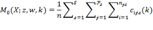
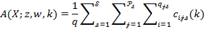
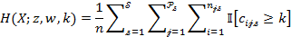
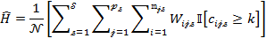
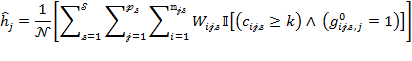
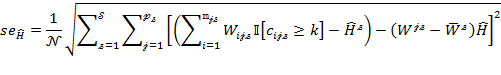
This appendix provides a technical outline of how standard errors may be computed. We first present the analytical approach and then the bootstrap method using the notation in Method I presented in Box 5.7. For the multidimensional and censored headcount ratios, we use the notation in Box 5.4. The ![]() and its partial indices are written as
and its partial indices are written as
|
|
|
|||
|
|
(8.6) |
|
||
|
|
(8.7) |
|
||
|
|
||||
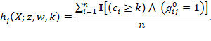
Note that ![]() is the logical ‘and’ operator. The standard errors of the subgroups’
is the logical ‘and’ operator. The standard errors of the subgroups’ ![]() s and partial indices may be computed in the same way and so we only outline the standard errors of equations (8.5)–(8.8).
s and partial indices may be computed in the same way and so we only outline the standard errors of equations (8.5)–(8.8).
Simple Random Sampling with Analytical Approach
Suppose ![]() samples have been collected through simple random sampling from the population. We denote the dataset by
samples have been collected through simple random sampling from the population. We denote the dataset by ![]() and its
and its ![]() th element by
th element by ![]() for all
for all ![]() and
and ![]() . We denote the deprivation status score for
. We denote the deprivation status score for ![]() by
by ![]() . For statistical inferences, our analysis focuses on the censored deprivation scores. The score, defined at the population level, becomes a random variable while performing statistical inference. We assume that a random sample (of size
. For statistical inferences, our analysis focuses on the censored deprivation scores. The score, defined at the population level, becomes a random variable while performing statistical inference. We assume that a random sample (of size ![]() ) of censored deprivation scores {
) of censored deprivation scores {![]() is a sequence of independently and identically distributed random variables with an expected value
is a sequence of independently and identically distributed random variables with an expected value ![]() and Var
and Var![]() . Then as
. Then as ![]() approaches infinity, the random variable
approaches infinity, the random variable ![]() converges in distribution to
converges in distribution to ![]() , where
, where ![]() . That is
. That is
|
|
(8.9) |
The unbiased sample estimate of ![]() is
is
|
|
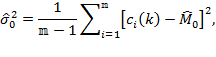
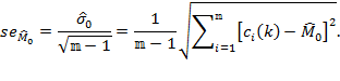
and the standard error of the Adjusted Headcount Ratio is
|
|
The analytical approach based on the central limit theorem (CLT) also applies to the calculation of the standard errors of ![]() , which leads to
, which leads to
|
|
(8.12) |
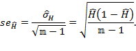
where ![]() and
and ![]() . Note that unlike
. Note that unlike ![]() ,
, ![]() is an average across 0s and 1s, i.e. the mean is a proportion and
is an average across 0s and 1s, i.e. the mean is a proportion and ![]() is estimated as
is estimated as
|
|
and so the unbiased standard error is
|
|
(8.14) |
With the same logic, the standard error for ![]() , can be estimated as
, can be estimated as
|
|
(8.15) |
where, ![]() .
.
The formulation of ![]() is analogous to the formulation of
is analogous to the formulation of ![]() , and so the standard error of
, and so the standard error of ![]() ) is computed as
) is computed as
|
|
where ![]() and
and ![]() is the number multidimensionally poor in the sample.
is the number multidimensionally poor in the sample.
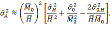
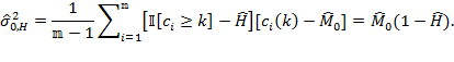
Note that if the number of multidimensionally poor is extremely low, the sample size for estimating ![]() may not be large enough. This may affect the precision of
may not be large enough. This may affect the precision of ![]() using (8.16). It may then be accurate to treat
using (8.16). It may then be accurate to treat ![]() as a ratio of
as a ratio of ![]() and
and ![]() for computing
for computing ![]() . By the Taylor series expansion (see the discussion in Casella and Berger 1990: 240–245),
. By the Taylor series expansion (see the discussion in Casella and Berger 1990: 240–245), ![]() can be approximated as
can be approximated as ![]() and
and ![]() can be estimated as
can be estimated as
|
|
where ![]() and
and ![]() are based on (8.10) and (8.13), respectively, and
are based on (8.10) and (8.13), respectively, and ![]() can be estimated as
can be estimated as
|
|
By combining (8.17) and (8.18), the alternative formulation becomes
|
|
(8.19) |
Stratified Sampling with an Analytical Approach
We next discuss the estimation of standard errors when samples are collected through two-stage stratification.[22] Using information on the population characteristics, the population is partitioned into several strata. The first stage, from each stratum, draws a sample of PSUs with or without replacement. The second stage draws samples either with or without replacement, from each PSU.
We suppose that the population is partitioned into ![]() strata and there are
strata and there are ![]() PSUs in the
PSUs in the ![]() th strata for all
th strata for all ![]() . The population size of the
. The population size of the ![]() th PSU in the
th PSU in the ![]() th stratum is
th stratum is ![]() so that
so that ![]() . We denote the total number of poor by
. We denote the total number of poor by ![]() and the number of poor in the
and the number of poor in the ![]() th PSU in the
th PSU in the ![]() th strata by
th strata by ![]() . The population
. The population ![]() measure and its partial indices are presented in (8.20)–(8.23) with the same notation for the identity function as in (8.5)–(8.8).
measure and its partial indices are presented in (8.20)–(8.23) with the same notation for the identity function as in (8.5)–(8.8).
|
|
||
|
|
(8.21) |
|
|
|
(8.22) |
|
|
|
Note that ![]() if the
if the ![]() th person from the
th person from the ![]() th PSU in the
th PSU in the ![]() th stratum is deprived in the
th stratum is deprived in the ![]() th dimension and
th dimension and ![]() otherwise; and
otherwise; and ![]() and
and ![]() are the deprivation score and the censored deprivation score of the
are the deprivation score and the censored deprivation score of the ![]() th person from the
th person from the ![]() th PSU in the
th PSU in the ![]() th stratum, respectively. Thus,
th stratum, respectively. Thus, ![]() ; and
; and ![]() if
if ![]() and
and ![]() otherwise.
otherwise.
Now, suppose a sample of size ![]() is collected through a two-stage stratified sampling. The first stage selects
is collected through a two-stage stratified sampling. The first stage selects ![]() PSUs from the
PSUs from the ![]() th stratum for all
th stratum for all ![]() . The second stage selects
. The second stage selects ![]() samples from the
samples from the ![]() th PSU in thstratum
th PSU in thstratum ![]() . So,
. So, ![]() . Each sample
. Each sample ![]() in the
in the ![]() th PSU in the
th PSU in the ![]() th stratum is assigned a sampling weight
th stratum is assigned a sampling weight ![]() , which are summarized by an
, which are summarized by an ![]() -dimensional vector
-dimensional vector ![]() . The achievements are summarized by matrix
. The achievements are summarized by matrix ![]() , which is a typical sample dataset.
, which is a typical sample dataset.
In order to estimate the measure from the sample, first, the total population and the total number of poor should be estimated from the sample. We denote the estimates of the population ![]() by
by ![]() and the estimate of the poor population
and the estimate of the poor population ![]() by
by ![]() . Then,
. Then,
|
|
(8.24) |
|
|
|
(8.25) |
The sample estimates of the population averages in (8.20)–(8.23) are presented in (8.26)–(8.29).
|
|
||
|
|
||
|
|
(8.28) |
|
|
|
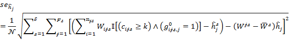
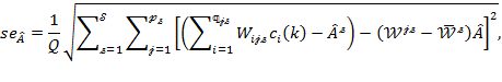
As each sample estimate is a ratio of two estimators, their standard errors are approximated using (8.17) and using equations (1.31) and (1.63) in Deaton (1997). The standard error for ![]() in (8.26) is
in (8.26) is
|
|
where ![]() ,
, ![]() and
and ![]() .
.
The standard errors of ![]() and
and ![]() are
are
|
|
|
||
|
|
|
||
(8.32)
where![]() and
and ![]() . Terms
. Terms ![]() and
and ![]() are the same as in (8.30).
are the same as in (8.30).
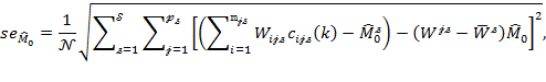
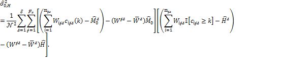
Finally, we present the standard error for ![]() in (8.27), where the denominator is
in (8.27), where the denominator is ![]() instead of
instead of ![]() as
as
|
|
where ![]() ,
, ![]() and
and ![]() . Intuitively,
. Intuitively, ![]() is the estimated average intensity for stratum
is the estimated average intensity for stratum ![]() ,
, ![]() is the average of sampling weights in stratum
is the average of sampling weights in stratum ![]() across the poor, and
across the poor, and ![]() is the sum of all sampling weights in PSU
is the sum of all sampling weights in PSU ![]() of stratum
of stratum ![]() also across the poor.
also across the poor.
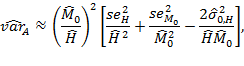
As a reasonably smaller sample size may affect the precision of the standard error of ![]() the variance
the variance ![]() can be approximated as in (8.17), but using (8.30) and (8.31) as
can be approximated as in (8.17), but using (8.30) and (8.31) as
|
|
where
|
|
|
(8.35)
Hence, combining (8.34) and (8.35), we have
|
|
(8.36) |
Note that the analytical standard errors and confidence intervals may not serve too well when the sample sizes are small or when the estimates are too close to the natural upper or lower bounds.[23] In these cases, resampling non-parametric methods, such as bootstrap, may be more suitable for computing standard errors and confidence intervals.
The Bootstrap Method
An alternative approach for statistical inference is the ‘bootstrap’, which is a data-based-simulation method for assessing statistical accuracy. Introduced in 1979, it provides an estimate of the sampling distribution of a given statistic ![]() , such as the standard error, by resampling from the original sample (cf. Efron 1979; Efron and Tibshirani 1993). It has certain advantages over the analytical approach. First, the inference on summary statistics does not rely on CLT as the analytical approach. In particular, for reasonably small sample size, standard errors/confidence intervals computed through the CLT-based asymptotic approximation may be inaccurate. Second, the bootstrap can automatically take into account the natural bounds of the measure. Confidence intervals using the analytical approach can lie outside natural bounds, which can be prevented when the bootstrap re-sampling distribution of the statistic is directly used.
, such as the standard error, by resampling from the original sample (cf. Efron 1979; Efron and Tibshirani 1993). It has certain advantages over the analytical approach. First, the inference on summary statistics does not rely on CLT as the analytical approach. In particular, for reasonably small sample size, standard errors/confidence intervals computed through the CLT-based asymptotic approximation may be inaccurate. Second, the bootstrap can automatically take into account the natural bounds of the measure. Confidence intervals using the analytical approach can lie outside natural bounds, which can be prevented when the bootstrap re-sampling distribution of the statistic is directly used.
Third, the computation of standard errors may become complex when the estimator and its standard error have a complicated form or have a no-closed expression. These types of complexities are common both in the context of statistical inference of inequality or poverty measurement and in tests where comparisons of group inequality or poverty (across gender or region) are of particular interest (Biewen 2002). Although, the delta-method can handle these analytical standard errors from stochastic dependencies, but when the number of time periods or groups increases, computing the standard errors analytically can easily become cumbersome (cf. Cowell 1989, Nygard and Sandström 1989). In practice, Monte Carlo evidence suggests that bootstrap methods are preferred for these analyses and shows that the simplest bootstrap procedure achieves the same accuracy as the delta-method (Biewen 2002; Davidson and Flachaire 2007). In developing economics, bootstrap has been used to draw statistical inferences for poverty and inequality measurement (Mills and Zandvakili 1997; Biewen 2002).
Here we briefly illustrate the use of the bootstrap for computing standard errors. Readers interested in using the bootstrap for confidence interval estimation and hypothesis testing can refer to Efron and Tibshirani (1993), chapters 12 and 16, respectively.
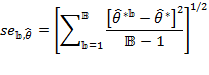
The bootstrap algorithm can be described as a resampling technique, which is conducted ![]() number of times by generating a random artificial sample each time, with replacement from the original sample, which is our dataset
number of times by generating a random artificial sample each time, with replacement from the original sample, which is our dataset ![]() . The
. The ![]() th resample produces an estimate
th resample produces an estimate ![]() for all
for all ![]() . Thus, we have a set of
. Thus, we have a set of ![]() resample estimates of
resample estimates of ![]() :
: ![]() . If the artificial samples are independent and identically distributed (i.i.d.), the bootstrap standard error estimator of
. If the artificial samples are independent and identically distributed (i.i.d.), the bootstrap standard error estimator of ![]() , denoted
, denoted ![]() , is defined as
, is defined as
|
|
(8.37) |
where ![]() stands for the arithmetic mean over the artificial samples. Even if the artificial sample is drawn from a more complex but known sampling framework, the bootstrap standard error can be easily estimated from standard formulas (cf. Efron 1979; Efron and Tibshirani 1993). If the resampling is conducted on an empirical distribution of a given dataset
stands for the arithmetic mean over the artificial samples. Even if the artificial sample is drawn from a more complex but known sampling framework, the bootstrap standard error can be easily estimated from standard formulas (cf. Efron 1979; Efron and Tibshirani 1993). If the resampling is conducted on an empirical distribution of a given dataset ![]() , then it is referred to as a non-parametric bootstrap. In this case, each observation is sampled (with replacement) from the empirical distribution, with probability inversely proportional to the original sample size. However, the resampling can also be selected from a known distribution chosen on an empirical or theoretical basis. In this case, it is referred to as a parametric bootstrap.
, then it is referred to as a non-parametric bootstrap. In this case, each observation is sampled (with replacement) from the empirical distribution, with probability inversely proportional to the original sample size. However, the resampling can also be selected from a known distribution chosen on an empirical or theoretical basis. In this case, it is referred to as a parametric bootstrap.

Box 8.1 illustrates the use of the bootstrap for computing standard errors of the ![]() and its partial indices. In this case, the statistic
and its partial indices. In this case, the statistic ![]() comprises
comprises ![]() ,
, ![]() ,
, ![]() , and
, and ![]() . Thus, the estimate
. Thus, the estimate ![]() includes
includes ![]() ,
, ![]() ,
, ![]() or
or ![]() . To obtain the bootstrap standard errors, we need to pursue the following steps.
. To obtain the bootstrap standard errors, we need to pursue the following steps.
- Draw
 bootstrap resamples from the empirical distribution function.
 - Compute the set of
 relevant bootstrap estimates of
  ,
,  ,
,  or
or  from each bootstrap sample.
 - Estimate the standard errors by the sampling standard deviation of the replications:
 ,
,  ,
,  , or
, or  (cf. Efron and Tibshirani 1993: 47).
We have already discussed that the bootstrap approach has certain advantages—especially that it does not rely on the central limit theorem. Although the non-parametric bootstrap approach does not depend on any parametric assumptions, it does involve certain choices. The first is the number of replications. Indeed a larger number of replications increas the precision of the estimates, but is costly in terms of time. There are different approaches for selecting the appropriate number of replications (see Poi 2004). The second involves the choice of the bootstrap sample size being selected from the original sample. The third involves the choice of the resampling method. The bootstrap sample size in Efron’s traditional bootstrap is equal to the number of observations in the original sample, but the use of smaller sample sizes has also been studied (for further theoretical discussions; see Swanepoel (1986) and Chung and Lee (2001).
Bibliography
Alkire et al. (2010): Alkire, S., Santos, M. E., Seth, S., and Yalonetzky, G. (2010). ‘Is the Multidimensional Poverty Index Robust to Different Weights?’ OPHI Research in Progress 22a, Oxford University.
Alkire, S. and Foster, J. (2011a). ‘Counting and Multidimensional Poverty Measurement’. Journal of Public Economics, 95(7–8): 476–487.
Alkire, S. and Santos, M. E. (2010). ‘Acute Multidimensional Poverty: A New Index for Developing Countries’. OPHI Working Paper 38, Oxford University; also published as Human Development Research Paper 2010/11.
Alkire, S. and Santos, M. E. (2014). ‘Measuring Acute Poverty in the Developing World: Robustness and Scope of the Multidimensional Poverty Index’. World Development, 59: 251–274.
Alkire, S. and Seth, S. (2013b). ‘Multidimensional Poverty Reduction in India between 1999 and 2006: Where and How?’ OPHI Working Paper 60, Oxford University.
Anderson, G. (1996). ‘Nonparametric Tests of Stochastic Dominance in Income Distributions’. Econometrica, 64(5): 1183–1193.
Barrett, G. and Donald, S. G. (2003). ‘Consistent Tests for Stochastic Dominance’. Econometrica, 71(1): 71–103.
Batana, Y. M. (2013). ‘Multidimensional Measurement of Poverty Among Women in Sub-Saharan Africa’. Social Indicators Research, 112(2): 337–362.
Biewen, M. (2002). ‘Bootstrap Inference for Inequality, Mobility and Poverty Measurement’. Journal of Econometrics, 108(2): 317–342.
Boland, P. J. and Proschan, F. (1988). ‘Multivariate Arrangement Increasing Functions with Applications in Probability and Statistics’. Journal of Multivariate Analysis, 25(2): 286–298.
Cherchye et al. (2007): Cherchye L., Moesen, W., Rogge, N., Puyenbroeck, T.V., Saisana, M., Saltelli, A., Liska, R., and Tarantola, S. (2007). ‘Creating Composite Indicators with DEA and Robustness Analysis: The Case of the Technology Achievement Index’. Journal of the Operational Research Society, 59(2): 239–251.
Cherchye et al. (2008): Cherchye L., Ooghe, E., and Puyenbroeck, T. V. (2008). ‘Robust Human Development Rankings’. Journal of Economic Inequality, 6(4): 287–321.
Chung, K. H. and Lee, S. (2001). ‘Optimal Bootstrap Sample Size in Construction of Percentile Confidence Bounds’. Scandinavian Journal of Statistics, 28(1): 225–239.
Cowell, F. (1989). ‘Sampling Variance and Decomposable Inequality Measures’. Journal of Econometrics 42(1): 27–41.
Davidson, R. and Duclos, J.-Y. (2000). ‘Statistical Inference for Stochastic Dominance and for the Measurement of Poverty and Inequality’. Econometrica, 68: 1435–1464.
Davidson, R. and Duclos, J.-Y. (2012). ‘Testing for Restricted Stochastic Dominance’. Econometric Reviews, 32(1): 84–125.
Davidson, R. and Flachaire, E. (2007). ‘Asymptotic and Bootstrap Inference for Inequality and Poverty Measures’. Journal of Econometrics, 141(1): 141–166.
Deaton, A. (1997). The Analysis of Household Surveys. A Microeconometric Approach to Development Policy. John Hopkins University Press.
Duclos, J.-Y. and Araar, A. (2006). Poverty and Equity: Measurement, Policy and Estimation with DAD. Springer.
Efron, B. (1979). ‘Bootstrap Methods: Another Look at the Jackknife’. The Annals of Statistics, 7(1): 1–26.
Efron, B. and Tibshirani, R. (1993). An Introduction to the Bootstrap. Chapman & Hall/CRC.
Foster J., McGillivray, M., and Seth, S. (2009). ‘Rank Robustness of Composite Indices’. OPHI Working Paper 26, Oxford University.
Foster, J. E., McGillivray, M., and Seth, S. (2013). ‘Composite Indices: Rank Robustness, Statistical Association and Redundancy’. Econometric Reviews, 32(1): 35–56.
Høyland et al. (2012): Høyland, B., Moene, K., and Willumsen, F. (2012). ‘The Tyranny of International Index Rankings’. Journal of Development Economics, 97(1): 1–14.
Joe, H. (1990). ‘Multivariate Concordance’. Journal of Multivariate Analysis, 35(1): 12–30.
Kendall, M. G. (1970), Rank Correlation Methods, London: Griffin.
Kendall, M. G. and Gibbons, J. D. (1990). Rank Correlation Method. E. Arnold.
Lasso de la Vega, M. C. (2010). ‘Counting Poverty Orderings and Deprivation Curves’, in J. A. Bishop (ed.), Studies in Applied Welfare Analysis: Papers from the Third ECINEQ Meeting. Research on Economic Inequality 18, ch. 7.
Mills, A.M. and Zandvakili, S. (1997). ‘Statistical Inference via Bootstrapping for Measures of Inequality’. Journal of Applied Econometrics, 12(2): 133–150.
Nardo et al. (2005): M., Saisana, M., Saltelli, A., Tarantola, S., Hoffman, A., and Giovannini, E. (2005). ‘Handbook on Constructing Composite Indicators: Methodology and User’s Guide’. OECD Statistics Working Papers 2005/3. OECD Publishing.
Newcombe, R. G. (1998). ‘Two-sided Confidence Intervals for the Single Proportion: Comparison of Seven Methods’. Statistics in Medicine, 17(8): 857–872.
Nygård, F. and Sandström, A. (1989). ‘Income Inequality Measures Based on Sample Surveys’. Journal of Econometrics, 42(1): 81–95.
Permanyer I. (2011). ‘Assessing the Robustness of Composite Indices Rankings’. Review of Income and Wealth 57(2): 306–326.
Permanyer, I. (2012). ‘Uncertainty and Robustness in Composite Indices Rankings’. Oxford Economic Papers 64(1): 57–79.
Poi, B. P. (2004). ‘From the Help Desk: Some Bootstrapping Techniques’. Stata Journal, 4(3): 312–328.
Saisana et al. (2005): Saisana, M., Saltelli, A., and Tarantola, S. (2005). ‘Uncertainty and Sensitivity Analysis as Tools for the Quality Assessment of Composite Indicators’. Journal of the Royal Statistical Society: Ser. A (Statistics in Society), 168(2): 307–323.
Seth, S. (2013). ‘A Class of Distribution and Association Sensitive Multidimensional Welfare Indices’. Journal of Economic Inequality, 11(2): 133–162.
Swanepoel, J. W H. (1986). ‘A Note on Proving that the (Modified) Bootstrap Works’. Communications in Statistics (Theory and Methods) 15(11): 3193–3203.
Ura et al. (2012): Ura, K., Alkire, S., Zangmo, T, and Wangdi, K. (2012). An Extensive Analysis of The Gross National Happiness Index. Centre of Bhutan Studies.
Wolff et al. (2011): Wolff, H., Chong, H., and Auffhammer, M. (2011). ‘Classification, Detection and Consequences of Data Error: Evidence from the Human Development Index’. The Economic Journal, 121(553): 843–870.
Yalonetzky, G. (2014). ‘Conditions for the Most Robust Multidimensional Poverty Comparisons Using Counting Measures and Ordinal Variables’. Social Choice and Welfare. Published online February.
[1] This chapter is confined to assessing the robustness of rank ordering across groups. Naturally it is essential also to assess the sensitivity of key values (such as the values of ![]() and dimensional contributions) to parameter changes, in situations in which policies use these cardinal values.
and dimensional contributions) to parameter changes, in situations in which policies use these cardinal values.
[2] There is a well-developed literature on robustness and sensitivity analyses for composite indices rankings with respect to relative weights, normalization methods, aggregation methods, and measurement errors. See Nardo et al. (2005), Saisana et al. (2005), Cherchye et al. (2007), Cherchye et al. (2008), Foster, McGillivray and Seth (2009, 2013), Permanyer (2011, 2012), Wolff et al. (2011), and Høyland et al. (2012). These techniques may require adaptation to apply to normative, counting-based measures using ordinal data.
[3] More elaborative dominance analysis can be conducted with respect to the deprivation cutoffs and weights. For multivariate stochastic dominance analysis using ordinal variables, see Yalonetzky (2014).
[4] In empirical applications, some statistical tests cannot discern between weak and strong dominance and thus assume ![]() first order stochastically dominates distribution
first order stochastically dominates distribution ![]() , if
, if ![]() for all
for all ![]() . See, for example, Davidson and Duclos (2012: 88–89).
. See, for example, Davidson and Duclos (2012: 88–89).
[5] This is also variously known as survival function or reliability function in other branches of studies.
[6] Technically, ![]() for poverty cutoff
for poverty cutoff ![]() can be expressed as
can be expressed as ![]() . In our example, Area I is computed as
. In our example, Area I is computed as ![]() and Area II as
and Area II as ![]() .
.
[7] In this book, we only focus on bivariate rank correlation coefficients, but there are various methods to measure multivariate rank concordance that we do not cover. For such examples, see Boland and Proschan (1988), Joe (1990), and Kendall and Gibbons (1990). For an application of some of the multivariate concordance methods to examine multivariate concordance of MPI rankings, see Alkire et al. (2010).
[8] The computations of the Spearman and Kendall coefficients in the table have been adjusted for ties. For the exact formulation of tie-adjusted coefficients, see Kendall and Gibbons (1990).
[9] Various sampling methods, such as simple random sampling, systematic sampling, stratified sampling, and proportional sampling, are used to conduct a sampling survey.
[10] Yalonetzky (2010).
[11] If the particular condition under study does not justify the assumptions made here, then these assumptions need to be relaxed and the standard error formulations are adjusted accordingly.
[12] The significance level is also referred to as the Type I error, which is the probability of rejecting the null hypothesis when it is true. See section 8.2.3 for the notion of null hypothesis. By statistical convention, the significance level is denoted with ![]() . However, to avoid confusion with the use of this symbol for other purposes in this book, we denote it
. However, to avoid confusion with the use of this symbol for other purposes in this book, we denote it ![]() .
.
[13] Whenever the population standard deviation is unknown or when the sample size is small, one needs to use the Student-t distribution to compute the critical values rather than the standard normal distribution.
[14] We present the tests for country-level estimates but they are equally applicable to other population subgroups. Also, we only present the tests in terms of the ![]() measure, but again they are also applicable to
measure, but again they are also applicable to ![]() ,
, ![]() and
and ![]() for all
for all ![]() and so we have chosen not to repeat the results.
and so we have chosen not to repeat the results.
[15] See Bennett and Mitra (2013) for an exposition of hypothesis testing of ![]() and other AF partial sub-indices using a minimum p-value approach.
and other AF partial sub-indices using a minimum p-value approach.
[16] See chapters 14 and 16 of Duclos and Araar (2006) for further discussion on non-independent samples for panel data analysis.
[17] Alkire and Seth (2013b) use an MPI harmonized for strict comparability of indicator definitions across time.
[18] For formal tests on stochastic dominance in unidimensional poverty and welfare analysis, see Anderson (1996), Davidson and Duclos (2000), and Barrett and Donald (2003).
[19] Other new ways of testing robustness may be developed in the near future.
[20] They compute the MPI for four population subgroups: children 0–14 years of age, women 15–49 years of age, women aged 50 years and older, and men 15 years and older, and test the rankings of subgroup MPIs across countries.
[21] Further methodological work is needed to propose overall robustness standards for measures that will be used for policy.
[22] Appendix D of Seth (2013) gives an example of standard error estimation for one-stage sample stratification in the multidimensional welfare framework; for consumption/expenditure see Deaton (1997).
[23] When the estimate is too close to the natural upper and lower bounds (0 and 1), the confidence intervals using analytical standard error may fall outside these bounds. Different methods for adjustments are available. For a discussion of such methods, see Newcombe (1998).