6 Normative Choices in Measurement Design
The modern field of inequality measurement grew out of the intelligent application of quantitative methods to imperfect data in the hope of illuminating important social issues. The important social issues remain, and it is interesting to see the ways in which modern analytical techniques can throw some light on what it is possible to say about them (Cowell 2000: 133).
Human beings are diverse in many and important ways: they vary in age, gender, ethnicity, nationality, location, religion, relationships, abilities, personalities, occupations, leisure activities, interests, and values. Poverty measures seek to identify legitimate, accurate, and policy-relevant comparisons across people, whilst fully respecting their basal diversity. Further, they seek to do so using data that are affected by several kinds of errors and limitations. This is no straightforward task.
After a measurement methodology has been chosen, the design of poverty measures—whether unidimensional or multidimensional—also require a series of choices. We turn to these now. The choices relate to the space of the measure, its purpose, unit of identification and analysis, dimensions, indicators, deprivation cutoffs, weights, and poverty line. Of these, ‘purpose’ is particularly influential in shaping the measure. As Ravallion states succinctly, ‘One wants the method of measurement to be consistent with the purpose of measurement’ (1998: 1). This chapter describes each of these normative choices in the context of multidimensional poverty measurement design and outlines alternative ways that these choices might be understood, made, and justified. Many normative theories or approaches might be used to inform measurement design, including human needs, objective lists, subjective wellbeing, human rights, and preference-based approaches, as well as many other less formally defined approaches.[1] Whichever are used, the normative contribution is not simply philosophical; it has a practical aim: to motivate poverty reduction.
Taken together, normative choices link the data and measurement design back to poor people’s lives and values and forward to the policies that, informed by poverty analysis, will seek to improve these. For example, dimensions which contribute disproportionately to poverty might become policy ‘priorities’. Do these reflect poor people’s values? Regions showing high poverty levels may be targeted geographically: does these accord with poor communities', taxpayers' and experts' understandings of who is poor? Programmes such as cash transfers may target households: do the poorest households benefit? The headlines (and political leaders) celebrate when multidimensional poverty falls—is this situation also applauded by those they seem to have assisted? It goes without saying that if the measure of poverty is unhinged from people’s voices and values, poverty policies are unlikely to hit the mark.
The normative choices inherent in monetary and multidimensional poverty design appear to cause consternation, particularly if measurement conventions have not yet been established.[2] In a section of The Idea of Justice named ‘The fear of non-commensurability’, Sen describes ‘non-commensurability’ as ‘a much-used philosophical concept that seems to arouse anxiety and panic’ (2009: 240). Yet setting priorities is no weakness. As Sen points out, ‘the need for selection and discrimination is neither an embarrassment, nor a unique difficulty, for the conceptualization of functionings and capabilities’ (1992: 46 and 44).
Building on Sen in their extremely relevant work Disadvantage, Wolff and De-Shalit elaborate additional conceptual insights that are relevant to address the ‘indexing problem’ in measurement. Defining poverty as clustered disadvantage, their policy goal is: ‘a society in which disadvantages do not cluster, a society where there is no clear answer to the question of who is the worst off. To achieve this, governments need to give special attention to the way patterns of disadvantage form and persist, and to take steps to break up such clusters’ (2007: 10). They argue that because disadvantages are interconnected and must be solved by policies that break up such clusters, and also because key policy decisions such as budget allocation require “some sort of overall assessment of disadvantage,” then “an overall index of disadvantage seems inescapable” (95, 89). They then proceed to address how such an index could be legitimately constructed, and we will return to their work in following sections.
Given that multidimensional poverty measurement remains a relatively new field of endeavour, a clear overview of the judgments and comparisons that normative choices draw upon, using the capability approach as a springboard, may prove useful.[3] To motivate the discussion we begin by sharing a birds-eye view of how the Adjusted Headcount Ratio  measure can—if a set of assumptions about the normative choices are fulfilled—reflect capability poverty.[4], [5]
6.1 The Adjusted Headcount Ratio: A Measure of Capability Poverty?
Suppose that there are a set of dimensions, each of which represent functionings or capabilities that a person might or might not have—things like being well-nourished, being able to read and write, being able to drink clean water, and not being the victim of violence. The deprivation profile for each person shows which functionings they have attained and in which they are deprived, and weights are applied to these dimensions that reflect the relative value of each among the set of dimensions. Suppose that there is considerable agreement regarding the value of achieving the deprivation cutoff level of these functionings, such that most people would achieve at least that level if they could. Furthermore, suppose that we can anticipate what percentage of people would refrain from such achievements in certain functionings—those who might be fasting to the point of malnutrition at any given time, for example. It is convenient but not necessary to assume that these indicators are equally weighted.[6] And let us assume that in identifying who is poor, the calibration of poverty cutoff  reflects these predictions of voluntary abstinence, as well as anticipated data inaccuracies, while recognizing that a sufficient battery of deprivations probably signifies poverty. Setting the cutoff in this way permits a degree of freedom for people to opt out if they so choose while seeking, insofar as is possible, to identify as poor people for whom the deprivations are unchosen. Applying such a poverty cutoff reduces errors in identification—for example by permitting people who would voluntarily abstain not to be identified as poor and avoiding identifying people as poor because of data inaccuracies. Among the poor, the more deprivations they experience, the poorer they are. Having identified who is poor, we construct the Adjusted Headcount Ratio (
 ).
).
How might such an reflect capability poverty? The key insight is this: in such a measure, a higher value of represents more unfreedom, and a lower value, less. Given that the set of indicators will be unlikely to represent everything that constitutes poverty, if each element is widely valued, and if people who are poor and are deprived in a dimension would value being non-deprived in it, then we anticipate that deprivations among the poor could be interpreted as showing that poor people do not have the capability to achieve the associated functionings. Thus would be a (partial) measure of unfreedom, or capability poverty.
As noted above, such an interpretation of relies on assumptions regarding the parameters:
a) Indicators measure or proxy functionings or capabilities
b) People generally value attaining the deprivation cutoff level of each indicator
c) The weights reflect a defensible set or range of relative values on the deprivations
d) The cross-dimensional poverty cutoff reflects ‘who is capability poor’.
Such an interpretation implicitly also relies upon assumptions about data quality and accuracy, and empirical techniques (that measures are implemented accurately). It has quite a restricted and uniform approach to values: for example, using a non-union poverty cutoff to permit ‘some’ abstinence from functionings.[7] But it might at least signal an avenue worth pondering.
In fact, as Box 6.1 elaborates more formally, under these conditions, our identification strategy and Adjusted Headcount Ratio can be related to Pattanaik and Xu’s signature work (1990), except that we now focus on unfreedoms rather than on freedoms. In their lucid and illuminating paper, Pattanaik and Xu elaborate on Sen’s claim that freedom has intrinsic value, thus that the extent of freedom in an opportunity set matters—independently of its relationship to preferences and utility. In developing this claim axiomatically they propose that the ranking of two opportunity sets in terms of freedom should depend only on the number of options present in each set.[8]
Sen, responding to Pattanaik and Xu (1990), observed that not every additional option (singleton) would contribute to an expansion of freedom–only those options that a person values and has reason to value. ‘The evaluation of the freedom I enjoy from a certain menu must depend to a crucial extent on how I value the elements included in that menu’. For example, ‘if a set is enlarged by including an alternative which no one would choose in relevant circumstances (e.g., being beheaded at dawn), the addition of that alternative may not necessarily be seen as a strict enhancement of freedom…’ (Sen 1991: 21 and 25). Nor would a deprivation in that negatively valued alternative be seen as impoverishing.
Our assumptions regarding the choice of parameters avoid Sen’s critique if each dimension of poverty reflects something that people value and have reason to value. Further, we follow Anand and Sen (1997), who argued that it may be easier to obtain agreement on the value of a small set of unfreedoms than an ample set of freedoms.[9] As Sen points out, ‘in the context of some types of welfare analysis, e.g. in dealing with extreme poverty in developing economies, we may be able to go a fairly long distance in terms of a relatively small number of centrally important functionings (and corresponding basic capabilities, e.g. the ability to be well nourished and well sheltered, the capability of escaping preventable morbidity and premature mortality, and so forth)’ (1992: 44–45; cf. 1985b).
Note that this capability interpretation of does not directly represent ‘unchosen’ sets of capabilities in a counterfactual sense (Foster 2010). Nor does it necessarily incorporate agency (Alkire 2007). Rather, in a manner parallel to Pattanaik and Xu, it interprets the deprivations in at least a minimum set of widely valued achieved functionings as unfreedom, or capability poverty (Box 6.1).
Naturally capability poverty measures that have different specifications and reflect different purposes could be constructed for the same society. There might be a child poverty measure or a capability poverty measure reflecting the values of a specific cultural group such as nomadic populations, or there might be a national capability poverty measure that reflects important deprivations about which there is widespread agreement across social groups. Thus the decision to measure capability poverty does not generate one unique measure; decisions as to the scope and purpose of the measure and the data sources guide measurement design even if the choice of space has been settled.
We also hasten to point out that many legitimate and tremendously useful measures could be constructed using  but located in a different space or in a mixture of spaces. These would not be measures of capability poverty but could be powerful tools for reducing capability poverty. For example, the dimensions might be resources such as service delivery (hopefully identifying whether marginalized groups have real access and clarifying the quality of the services). The point is that our measurement framework can be used for different purposes including those unrelated to capabilities. So it is vitally important (and not terribly difficult) to articulate and explain the purpose of each application and to justify the choices and calibration of parameters.
This section set out the circumstances in which may measure capability poverty. The assumptions regarding values and data that must be fulfilled to do so were transparently stated. Under this interpretation, embodies a rather rudimentary kind of freedom; there could be many interesting extensions — for example, incorporating agency and process freedoms. Also, measures that do not reflect capability poverty will fulfil some purposes splendidly. Still, if the assumptions articulated here are fulfilled, we can indeed offer as a measure of capability poverty. For what is needed in this context is not a quixotic search for the perfect measure but rather methodologies that may be sufficient to advance critical ethical objectives. Most empirical outworkings of the capability approach have used drastic simplifications, and these can often be cheered as true advances, even while their limitations are borne in mind. ‘In all these exercises, clarity of theory has to be combined with the practical need to make do with whatever information we can feasibly obtain for our actual empirical analyses. The Scylla of empirical overambitiousness threatens us as much as the Charybdis of misdirected theory’ (Sen 1985: 49). In this sense, our methodology may be a step forward in operationalizing the measurement of capabilities.
Box 6.1 Unfreedoms and 
Let  be a poverty methodology satisfying decomposability, weak monotonicity, non-triviality, and ordinality.
The first three properties are satisfied by all members of methodology  ; however,
  is the only adjusted Foster–Greer–Thorbecke (FGT) measure that satisfies ordinality, and it is this property that ensures that its poverty levels and comparisons are meaningful when the dimensional variables are ordinal.
By decomposability, the structure of  depends entirely on the way that measures poverty over singleton subgroups; and by dichotomization, this individual poverty measure can be expressed as a function
  of the individual’s deprivation vector
  (which is any row
  of deprivation matrix
  ). In the case of
  , we have
  , where
  is the censored distribution defined as
  if
if  and
and  if
if  . We will now explore the possible forms that
  can take for dichotomized measures. Note that while the definition of
  is based in part on the dimensional cutoff
  , we have not specified the identification method employed by the general index
  . Hence a second question of interest is what forms of identification might be consistent with various properties satisfied by .
The individual poverty function for has two additional properties of interest. First, it satisfies anonymity or the requirement that  , where
  is any
  permutation matrix. This property implies that all dimensions are treated symmetrically by the poverty measure. Second, it satisfies semi-independence, which states that if
  , and
, and  , then
  .[10] Under this assumption, removing the same dimensional deprivation from two deprivation vectors should preserve the (weak) ordering of the two. We have the following result:
Let be the individual poverty function associated with a dichotomized poverty measure. satisfies anonymity and semi-independence if and only if there exists some  such that for any deprivation vectors and
  we have:
  if and only if
  .
.
In other words, ranks individual deprivation vectors in precisely the same way that does for some . This result is especially powerful since it simultaneously determines both the individual poverty index ( associated with the Adjusted Headcount Ratio  and the identification method (based on a dimensional cutoff ) consistent with the assumed properties. To establish the result we extend the generalization of Pattanaik and Xu given in Foster 2010. In particular, if full independence were required, so that the conditional in semi-independence were converted to full equivalence, then a direct analogue of the Pattanaik and Xu result would obtain, namely, if and only if
  . In this specification, would make comparisons of individual poverty the same way that the union-identified
  does—by counting all deprivations.
While our result uniquely identifies the individual poverty ranking, it leaves open a multitude of possibilities for the overall index  —one for each specific functional form taken by . For example, the individual poverty function
  , when averaged across the entire population to obtain , would place greater emphasis on persons with many deprivations. It would be interesting to explore alternative forms for and the properties of the associated index . Note that because of dichotomization, each of these measures would provide a way of evaluating multidimensional poverty when the underlying variables are ordinal.
Given the arguments in Foster 2010, it is straightforward to establish the above result. In particular, let  or
or  for all
  be the set of all individual deprivation vectors, and let
  be an individual poverty function associated with a standard dichotomized poverty measure such that satisfies anonymity and semi-independence. By anonymity, all vectors
  with
with  must satisfy
  . In other words, the value of depends entirely on the number of deprivations in . Weak monotonicity implies that
  for
for  , and so the value of is weakly increasing in the number of deprivations in . By non-triviality and decomposability, it follows that
  for
for  .[11] Let be the lowest deprivation count for which is strictly above
  ; in other words,
  for , and for . Semi-independence ensures that must be increasing in the deprivation count above . For suppose that for with
  . Then by repeated application of anonymity and semi-independence, we would have for some with
  , a contradiction. It follows, then, that
  is constant in
  for and increasing in for
  . Clearly, this is precisely the pattern exhibited by the function
  .
.
6.2 Kinds of Normative Choices
It may be asked whether choices underlying measurement design are normative and, if so, in what sense? If data are constrained and exactly one educational variable exists, in what sense is its selection normative? Similarly, if an indicator is redundant or invalid according to statistical assessments, how is its deselection normative? And if nutritional experts judge that an indicator of stunting is more accurate than wasting, in what way is a choice in its favour normative?
Normative considerations operate at different levels. Releasing a measure rather than not doing so may reflect a high-level normative judgement that releasing the measure is more likely to improve welfare than not releasing it.[12] This assessment may be made after consideration of what Sen (2009) terms a ‘comprehensive’ description of the situation. At a lower level, in each part of measurement design, value judgements are used to justify particular choices—like dimensions, weights, and poverty cutoffs. The value judgements may pertain to the content directly, or they may address the methodologies or processes by which to justify design choices, as later sections will illustrate.
At this higher meta-level, the comprehensive description and its normative assessment will draw upon different kinds of analyses—statistical, axiomatic, deliberative, practical, and policy-oriented, for example—to authorize the use of measures that fulfil a set of plural purposes reasonably well.
These higher level reasoned judgements that draw on a comprehensive description of the options often include the following types of assessments:
Expert (including qualitative) assessments of indicator accuracy—for example, in showing the level and changes of a key functioning like nutrition (Svedberg 2000) or the quality and legitimacy of a participatory process;
Empirical assessments, which could include analyses of measurement error, data quality, redundancy, robustness, statistical validity and reliability, or triangulation with other analyses and data sources;
Deliberative insights on people’s values from participatory discussions, social movements, consultations, and from documentation of similar recent processes;
Theoretical assessments, which could consider properties and principles, sets of dimensions, standards or conventions on indicators, or legal and policy frameworks;
Practicalities such as constraints of data, time, human resources, authority, political will, and political feasibility given the processes and authorities involved; and
Policy relevance—for example, how the timing and content of the measure could dovetail with resource allocation decisions or how a measure might support and monitor a set of planned interventions as set out in a national plan or a current campaign.
This section introduces this meta-coordination role of normative reasoning; later sections describe how particular kinds of assessment mentioned already may inform particular design choices.
The higher normative function is inextricably linked to the purpose(s) of the measure, which are often multiple and normally motivate policy and public action. As Foster and Sen put it, ‘The general conclusion that seems irresistible is that the choice of a poverty measure must, to a great extent, depend on the nature of the problem at hand’ (1997: 187).
A relevant example is Mexico’s move towards a multidimensional poverty measure. In his book Numbers that Move the World, Miguel Székely points out that:
Just like there are ideas that move the world, so too there are numbers and statistics that move the world. A number can awaken consciences; it can mobilize the reluctant, it can ignite action, it can generate debate; it can even, in the best of circumstances, lay to rest a pressing problem (2005: 13).[13]
In describing Mexico’s steps towards new options of poverty measurement, Székely describes how a committee was formed whose mandate was ‘to propose to the Secretary of Social Development a methodology that could be officially adopted as an instrument of the Mexican government to measure the magnitude of poverty, its intensity, and its characteristics’ (Székely 2005: 17). In 2001, the committee invited three international experts, including James Foster; and Foster, together with John Iceland and Robert Michael, identified the following desiderata that the proposed measurement methodology should fulfil — criteria that the committee adopted in its subsequent work:
- It must be understandable and easy to describe
- It must reflect ‘common-sense’ notions of poverty
- It must fit the purpose for which it is being developed
- It must be technically solid
- It must be operationally viable—e.g. in terms of data requirements
- It must be easily replicable (Székely 2005: 10 and 19).[14]
As these criteria suggest, there are usually plural desiderata for a measure, and these must be taken into account within a coordinating normative framework.[15] Consider the first purpose: a measure should be simple and easy to communicate. Earlier we observed that the widely used headcount ratio of income poverty lacks some very desirable properties. Indeed, because the headcount ratio ‘ignores the “depth” as well as the “distribution” of poverty’, Foster and Sen found it ‘remarkable that most empirical studies of poverty tend, still, to stop at the head-count ratio’ (1997: 168 and 169). On the other hand, when formulated as a criterion, it becomes evident that this characteristic — that a measure not only be axiomatically sound and empirically solid, but also easy to understand — is actually essential if the measure is to inform and engage public debate and policy.
Returning to the income poverty headcount ratio, it seems that the desirability of certain properties is balanced against ease of communication. For measures whose purpose is to incite public action, the choice to favour communication is comprehensible. Indeed the development of the Human Development Index, as Sen describes it, was largely driven by this need of communicability. Sen recounts how Mahbub ul Haq, the director of the then newly created Human Development Report Office of the United Nations Development Programme called for an index ‘of the same level of vulgarity as the GNP—just one number—but a measure that is not as blind to social aspects of human lives as the GNP is’ (Sen 1998). Properties vs. communicability is not the only trade-off: at times statistical accuracy and non-sampling measurement error may need to be balanced with ‘common sense’, or an ideal measure tempered by the need to use existing data.
The ‘higher’ or coordinating normative reasoning creates a ‘comprehensive’ description of possible measures according to the criteria, rules out options that are strictly worse than others, and identifies their relative strengths and challenges.[16] Even if, as is likely, the final choice of a multidimensional poverty measure is but one of a set of candidate measures, each of which is defensible and cannot be further ranked, the criteria will still have worked to eliminate measures that may have been less comprehensible and violated more key properties—or had higher measurement error, lower robustness and less policy salience than the ones that remain. They will also have identified the strengths and challenges of each candidate, and so the selection among them is essentially also a selection of which criteria to prioritize—a choice that will have been simplified by a clear analysis. For example, a society may wish to prioritize a measure that has legitimacy because it transparently draws on public consultations, which are important because recent history had discredited poverty statistics (so prioritizing criteria 2), or a measure that will incentivize policies because it is closely tied to a popular national plan (criteria 3) and so on.
In sum, multidimensional poverty measurement can seem rather bewildering at first because its justification may draw on axiomatic, statistical, ethical, data-related, deliberative/participatory, policy-oriented, political, and historical features. But in practice poverty measurement is considerably more concrete (Anand and Sen 1997, Alkire 2002b). The available resources and actual constraints – from timing to data to funding to political demand – for a given exercise often provide considerable structure and guidance. Thus, although normative engagement is required to coordinate various considerations, ‘there is no general impossibility here of making reasoned choices over combinations of diverse objects’ (Sen 2009: 241).
6.3 Elements of Measurement Design
The Alkire-Foster methodology is a general framework for measuring multidimensional poverty – an open-source technology that can be freely altered by the user to best match the measure’s context and evaluative purpose. As with most measurement exercises, it will be the designers who will have to make and defend the specific decisions underlying the implementation, limited and guided by the purpose of the exercise and other concrete constraints.
Traditional unidimensional measures require a set of parallel decisions with normative content.[17] For example, should the variable be expenditure or income? What indicators should comprise the consumption aggregate? How should ‘missing’ prices be set? What should the poverty line(s) be? If it reflect a food basket, how many calories should it total, and should it exclude cheap unhealthy foods? Choices to create comparability can likewise be important for final results, such as the construction of Purchasing Power Parity values or urban–rural adjustments, or adjustments for inflation. Robustness standards are crucial for all poverty measures, as they ensure that the results obtained are not unduly dependent upon the calibration choices (whether these are normatively based or not).[18]
The flexibility in AF measurement design means that measures at the country or subnational level can be designed to embody prevailing priorities or norms of what it means to be poor. For example, if dimensions, weights, and cutoffs are specified in a legal document such as the Constitution, the identification function might be developed using an axiomatic approach, as was done in Mexico.[19] Qualitative and participatory work can (and in our view should) triangulate other analyses.[20] The weights can also be developed by a range of processes: expert opinion, or coherence with a consensus document such as a national plan, focus groups, survey data, or human rights. And the poverty cutoff, which is analogous to poverty lines in unidimensional space, could be chosen so as to reflect poor people’s assessments of who is poor, as well as wider social assessments.
This section introduces the purpose of a poverty measure and the normative choices that inhere in measurement design.[21] We cover eight design elements. The first five serve to structure a poverty measure; the last three calibrate key parameters (cutoffs and weights).
- Purpose(s) of the measure: The purpose(s) of a measure may include its policy applications, the reference population, dimensions, and time horizon.
- The choice of space: The choice of space determines whether poverty is measured in the space of resources, inputs and access to services, outputs, or functionings and capabilities.
- The unit(s) of identification and analysis: These are unit(s) for which the AF method reflects the joint distribution of disadvantages, identifies who is poor, and analyses poverty.
- Indicators: Indicators are the building blocks of a measure; they bring into view relevant facets of poverty and constitute the columns of the achievement and deprivation matrices.
- Dimensions: Dimensions are conceptual categories into which indicators may be arranged (and possibly weighted) for intuition and ease of communication.
- Deprivation cutoffs: The deprivation cutoff for an indicator shows the minimum achievement level or category required to be considered non-deprived in that indicator.
- Weights: The weight or deprivation value affixed to each indicator reflects the value that a deprivation in that indicator has for poverty, relative to deprivations in the other indicators.
- Poverty cutoff: The poverty cutoff shows what combined share of weighted deprivations is sufficient to identify a person as poor.
In practice, these design choices are not made in a linear fashion but rather iteratively, and in combination with consultations and empirical work. Thus discussing them sequentially may seem rather tedious. Just like it is far more pleasant to hear a horse whinny than to transcribe its whinny painstakingly onto a musical staff to learn how it is done, so too, considering these choices one by one makes the task seem rather dull. One can only hope the transcription is a one-time task, whereas the skill of whinnying lasts awhile.
6.3.1 Purpose(s) of a Measure
The purpose(s) of a measure clarify the way(s) in which the measure will be used to describe and understand situations, to make comparisons across groups or across time, and to guide policy or monitor progress. The purpose shapes the choice of space and many of the calibration decisions that will follow and so should be explicitly formulated and stated. The Stiglitz–Sen–Fitoussi Commission drew attention, in the case of quality of life measures, to the fundamental importance of the purpose of the measure to the identification of dimensions and indicators. ‘The range of objective features to be considered in any assessment … will depend on the purpose of the exercise … the question of which elements should belong to a list of objective features inevitably depends on value judgements …’ (2009).
The purpose may also identify constraints and shape processes. For example, if the purpose includes legitimacy to the wider public, then public consultations may be essential; if it is performance monitoring, involvement with the concerned agencies and institutions may be useful. While a measure may have a single purpose, it is more common for measures to seek to fulfil multiple purposes.
For example, a national poverty measure might be used to assess the population-wide levels and trends in capability poverty across regions and population groups in ways that are regarded as legitimate and accurate by the citizenry. Note that this statement of purpose has scope (population-wide), space (capability), relevant comparisons (across population groups and time trends), and popular legitimacy (which affects procedures). A study may design a youth poverty measure in order to understand, profile, and draw attention to youth capabilities at a given point in time. A targeting measure may use census data to identify and target the poorest of the poor in terms of social rights for certain services. A performance monitoring measure may track changes over time across a set of indicators reflecting the goals of a programmatic intervention, such as improvement in the quality of education, or women’s empowerment across various domains. A local community development measure may monitor a village development plan in ways that community members have proposed and understand. Measures might be designed to inform the private sector and civil society about the state of poverty in their country and so encourage public debate. They might also clarify what value-added their analyses have in comparison with monetary poverty measures.
The purpose of the measure will often also include political economy and institutional issues and constraints that are pertinent to the measure fulfilling its purpose, such as timescale, data, budgetary resources, political and legal procedures, updating procedures and so on.[22] For example, will a given dataset be used or will a new survey be designed and implemented and if so what is its budget and frequency? Are particular committees, commissions, or institutional processes to be involved in measurement design and what is their authority? If a measure will be updated over time, what is its legal or institutional basis, which institution(s) or person(s) have the authority to update the measure, and when and how is occasional methodological updating to take place? Clarity on such issues can greatly streamline design procedures.
6.3.2 Choice of Space
As mentioned in section 6.1 another preliminary choice is the space in which that measurement is to proceed. Will it be in the space of income, of resources and access to resources, of functionings and capabilities, or of subjective utility? There are well-known arguments in favour of each space, and purposes for which each space might be appropriate. Conceptually it is vital to be clear about the choice of space prior to the selection of indicators. This is because the same indicators – such as years of schooling – may be used in empirical measures of both types, but the interpretation and, at times, the treatment of the data may vary.
Following Sen, we may take the space that is of central interest to be the space of functionings and capabilities (they are the same space). Functionings are the beings and doings that people value and have reason to value, and capabilities are the freedoms to achieve valuable functionings. This implies that measurement should focus on valuable activities and states of being that people actually achieve, given their values and their varying abilities to convert resources into functionings. The choice of space may have implications for the interpretation of variables’ scales of measurement. In some cases, measures use indicators that reflect achievements in other spaces (or subjective and self-reported states), if these can be justified empirically as proxies of functionings or capabilities.
An essential step at this stage is to revisit the scales of measurement introduced in section 2.3. To summarize, any achievement matrix may contain data having categorical, ordinal, or cardinal scales (which may be binary, interval, or ratio scale). In measures requiring cardinal data the indicator’s scale of measurement has to be reassessed after the space of measurement has been chosen. For example, years of schooling may seem to be a ratio-scale variable. But in terms of human functionings, is it? Or do the earlier years of education confer marginally more capabilities than later years, or the completion of the twelfth year (with a diploma) than the eleventh year (without a diploma)? In using , we dichotomize variables at a deprivation cutoff. This obviates the need to rescale indicators to construct an appropriate normalized gap in different spaces, but still requires that the deprivation cutoffs (discussed in section 6.3.6) reflect deprivations in the chosen space.
Not all measures focus on the capability space—or need to. They might reflect social rights, social exclusion, access to services, social protection, or the quality of services. And most poverty reduction requires, as intermediary steps, institutions that effectively deliver resources and services to people and communities. Thus even if the goal is capability expansion, this might be stimulated or monitored in part by a multidimensional poverty measure that is framed in an intermediary space of inputs or outputs. The choice of space specifies how a given measure will advance the purpose.
6.3.3 Units of Identification and Analysis
The unit(s) of identification or analysis[23] may be a person, a household, a geographic area, or an institution (such as a school or firm or clinic). A common unit of identification for a poverty measure is a person (any adult, a child, a worker, a woman, an elderly person). This permits a poverty measure to be decomposed by variables like gender, age, ethnicity, occupation, and other relevant individual characteristics. It may also permit analysis of intra-household patterns of poverty or of group-specific poverty (indigenous groups, youth unemployed, urban slums). Alternatively, household members’ information may considered together, which has advantages in terms of supporting intra-household sharing, and also at getting an overview of households. In this case, household members’ combined achievements are used as a unit of identification for a population-wide measure, and all household members receive the same deprivation score.
The unit of analysis – meaning how the results are reported and analysed – may still reflect each person. That is, even if the unit of identification is the household, one can report the percentage of people who are identified as poor (by using individual sampling weights), rather than the percentage of households that are identified as poor (which is used if the household is the unit of analysis).
Where data are not available at the household level or where the measure focuses on topics such as infrastructure, poverty can be computed for data zones or geographic areas, so long as there is a justification for overlooking within-region inequality. Other measures may use a particular institution such as a school or clinic or firm as a unit of identification and/or analysis.
What is essential is that data for all variables must be available for (or transformed to represent) each unit of identification (see also Chapter 7), that the definition of applicable populations be transparent and complete, and that the unit of analysis be explicitly and clearly stated and justified.
There are ethical considerations in choosing and justifying a unit of analysis. For example, using the person as the unit of identification coheres with human rights policies, can show gendered or age disparities, and may permit intra-household analysis (Alkire, Meinzen-Dick, et al. 2013). Yet using the household as a unit of identification acknowledges intra-household caring and sharing—for example, educated household members reading for each other, and multiple household members being affected by someone’s severe health conditions. Policies targeting or addressing the household may also strengthen or at least not weaken the household unit. Normative and policy assessments may be supplemented by participatory insights regarding the appropriate unit of identification and the ensuing focus of policy interventions.
The justification of a unit of identification may include empirical assessments of bias and comparability. For example, if the unit of identification is the household, then indicators that draw on individual-level achievements may be checked for biases according to household size and composition (Alkire and Santos 2014). If the unit of identification is the person, then the comparability of indicators across diverse groups requires analysis—as in the case of education and health indicators for people of different ages (infants and toddlers, school-aged children, adults, and the elderly). The scale of errors that could be introduced if household-level variables are presumed to be equally shared by all household members is a further fruitful topic of empirical scrutiny.
For some policy purposes it could be useful to construct a set of measures, in which each measure takes a nested unit of identification that includes or is included by related measures: for example, the person, the household, the village or neighbourhood, and the district. The ‘nested’ measures permit further analysis of the interactions between deprivations at different levels. For example, the individual-level data may have health and educational functionings, household data may have living standard and housing-related functionings, and village-level data may have environmental, infrastructure, and service delivery information. Analyses may explore the extent to which health- and education-deprived people live in living-standard-deprived households, for example, and whether these live in services-deprived villages. Alternatively one may study which poor children live in poor households. Analyses using nested measures can be compared to analyses of a multidimensional poverty index at the individual level that applies relevant household- and village-level deprivations to each individual.
In sum, although often data constraints will require that the household be the unit of identification, when other options are feasible, then this choice can be considered, made, and justified using different kinds of reasoning to assess the ‘fit’ between the proposed measure and its purpose.
6.3.4 Dimensions
When these structural choices have been established, poverty measures require the selection and valuation of deprivations. Sen introduces the task as follows: ‘In an evaluative exercise, two distinct questions have to be clearly distinguished: (1) What are the objects of value? (2) How valuable are the respective objects’ (Sen 1992: 42). These two tasks of selecting focal deprivations (using dimensions, indicators, and cutoffs) and setting relative values for them, recur in poverty measurement.
The term ‘dimensions’ in this chapter refers to conceptual categorizations of indicators for ease of communication and interpretation of results. By ‘indicators’ we mean the d variables that appear in columns of the achievement and deprivation matrices and are used to construct the deprivation scores and to measure poverty.
A multidimensional poverty measure is constructed using indicators. In some cases, these indicators may each represent distinct facets of poverty. In other cases, it may be useful to talk about several indicators as forming a ‘dimension’ of poverty. Why use dimensions? Dimensions may reflect the categories defined by some deliberative or synthetic processes. For example, a dimension might be children’s education; indicators might include a child’s years of completed schooling and their achievement scores last period. In this case the indicators may be the best possible approximation of those dimensions from an existing dataset. It may also arise from a theory or policy source. Noll (2002) develops a systematic conceptual framework for social indicators in Europe by reviewing concepts of welfare and common policy goals, then identifying fourteen dimensions that fit the measurement’s purposes. Grouping indicators into dimensions may facilitate the communication of results because there are likely to be fewer dimensions than indicators and they are likely to be intuitive and accessible to non-experts.
Grusky and Kanbur argue that the selection of dimensions merits active attention because ‘economists have not reached consensus on the dimensions that matter, nor even on how they might decide what matters’ (2006: 12). Yet the extensive and historic discussions about the post-2015 development agenda have been tremendously useful in illuminating areas of agreement across different interest groups with respect to widely varying national and international considerations.
Unusually, the selection of dimensions does not necessarily rely on empirical or technical analysis. Naturally sometimes analysts explore or confirm the extent to which dimensional grouping of indicators is corroborated statistically. Such statistical explorations should not determine the selection of dimensions or grouping of indicators; they may, however contribute to their justification and expose interesting relationships that should be considered.
In addition to the inevitable consideration of data constraints, there are at least three overlapping kinds of information that may inform the selection of dimensions: deliberation and public reasoning, legitimate consensus, and theoretical arguments (Alkire 2008a).
The first approach is a repeated deliberative or participatory exercise, which engages a representative group of participants as reflective agents in making the value judgements to select focal capabilities. Deliberation may involve online assessments as well as face-to-face focus groups; it may also consolidate the body of recent and similar participatory work that has been undertaken for other purposes. In a supportive, well-informed, and equitable environment, participatory processes seem to be ideal for choosing dimensions; not, however, if deliberation is dominated by conflict or inequality or misinformation, or coloured by the absence or dominance of certain groups. Furthermore, the process of aggregating the values of a diverse assembly of groups and people, whose deliberative processes may vary in quality, is neither elementary nor void of controversy (indeed it is an appropriate topic for further research). Even if a new set of deliberative exercises are not possible, it may be possible to consider documentation of previous such processes, be it from a previous measurement consultation, participatory exercises, a widely debated national plan, high-profile legal documents, the media, or a respectable set of life histories of disadvantaged people and communities (Leavy et al. 2013, Narayan et al. 2000). So it may be rare for a set of dimensions to be justified without any reference to participatory studies and public debates.
In writing on the selection of capabilities – which relate to dimensions and indicators[24]—Sen calls for deliberative engagement rather than using a pre-ordained list. ‘I have nothing against the listing of capabilities,’ Sen writes, ‘but must stand up against a grand mausoleum to one fixed and final list of capabilities’ (2004: 80). A central reason against promulgating a fixed list is that to be relevant, the dimensions (and indicators) should reflect the purpose of the measure. ‘What we focus on cannot be independent of what we are doing and why’ (Sen 2004: 79). The deprivations in international measures will rightly differ from a national measure or a measure of child poverty or of an indigenous community, for example. A further motivation for not fixing a list of capabilities even for a given purpose—including poverty measurement—is that a fixed list would crowd out debate and public reasoning, which can play an educational and motivational role. It also would not catalyze constructive debate that may influence people’s values. ‘To insist on a fixed forever list of capabilities would … go against the productive role of public discussion, social agitation, and open debates’ (Sen 2004: 80). Also, as technology advances and social values change, the list might become outdated (Sen 2004: 78). For example recent approaches to poverty often incorporate environmental and energy considerations that were lacking previously.
A second approach to the selection of dimensions is the use of an authoritative document or list that has attracted a kind of enduring consensus and associated legitimacy. Examples include a constitution, a national development plan, a declaration of human rights, or some time-bound international agreements such as the MDGs. Most official multidimensional poverty measures have some transparent link to such a policy process or document. The use of a set of dimensions that already have a kind of visibility and legitimacy is useful for international or global measures (where public deliberation is difficult), as well as for those that are clearly designed to monitor policy processes. It also naturally connects measurement to policy management.
A third potential source of dimensions is a conceptual framework or particular theory—which may range from Maslow’s hierarchy of human needs to a religious framework such as the Maqasid A-Sharia, to lists like Martha Nussbaum’s set of central human capabilities. These approaches are particularly relevant for communities where the theory enjoys widespread approval and/or is consistent with lists generated by alternative theories or processes (Alkire 2008a).
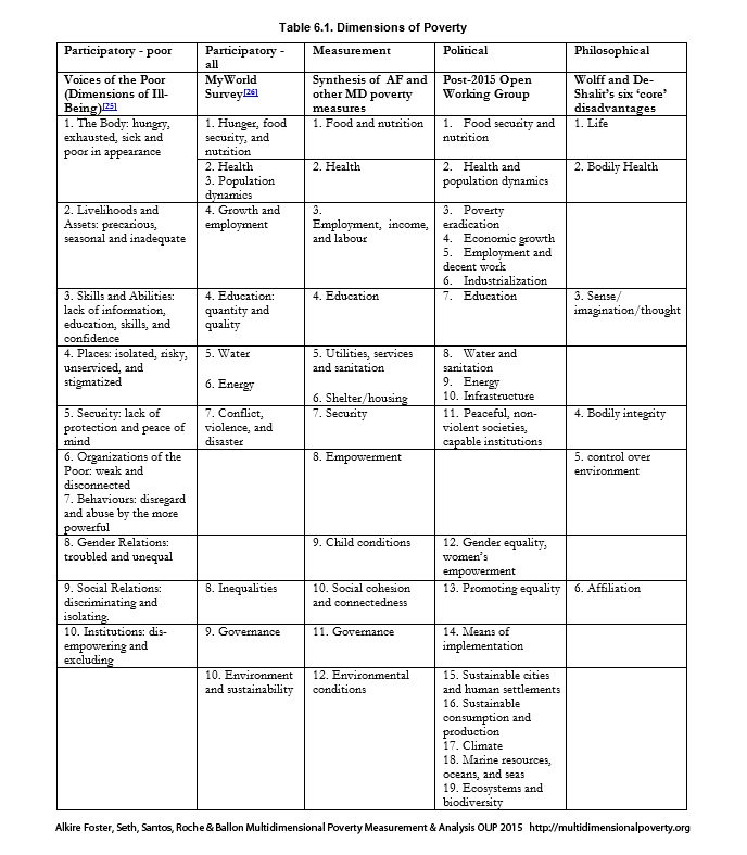
Comparing the lists that groups generate by these and additional processes, one finds a striking degree of commonality between them. Table 6.1 lists dimensions generated by these processes that pertain to multidimensional poverty measurement. Indeed there are a plethora of similar resources for the selection of deprivations, which may contribute towards standards supporting multidimensional poverty measurement design. And whilst the particular names and grouping of indicators differ, the universe of options is not too great, and this fact itself may be of no little comfort to those designing multidimensional poverty measures.
It should be borne in mind that the selection of dimensions and indicators affects the selection of weights. In a book supporting the development of national poverty plans in Europe, Tony Atkinson and colleagues point out the convenience of keeping weights in mind when selecting dimensions and indicators. In particular, they commend choosing indicators (or, possibly, dimensions) such that their weights are roughly equal to facilitate policy interpretations: ‘the interpretation of the set of indicators is greatly eased where the individual components have degrees of importance that, while not necessarily exactly equal, are not grossly different’ (Atkinson et al. 2002). Sen also emphasizes the interconnection between these choices: ‘There is no escape from the problem of evaluation in selecting a class of functionings in the description and appraisal of capabilities, and this selection problem is, in fact, one part of the general task of the choice of weights in making normative evaluation’ (Sen 2008). Elsewhere we observed that this linkage holds not only for dimensions that are selected but also for those that are omitted: ‘choosing one out of several possible variables is tantamount to assigning that dimension full weight and the remaining dimensions zero weight’ (Alkire and Foster 2011b). And it is to the selection of indicators that we now turn.
6.3.5 Indicators
Indicators are the backbone of measurement. Their quality, accuracy, and reach determine the informational content of a poverty measure. Given data constraints the process through which these are selected may include participatory and deliberative exercises, legal or political documents, statistical explorations, robustness tests, or theoretical guidelines.
While a considerable amount of attention, discussion, and practice has focused on the normative selection of dimensions of poverty and wellbeing, there is a paucity of comparable normative literature on the selection of indicators. The literature on indicator selection is, however, richly arrayed with a plethora of empirical considerations, which must be considered alongside normative and policy issues. Some of these will be raised in Chapter 7. These include:
- statistical techniques to assess aspects such as the reliability, validity, robustness, and standard errors of economic and social indicators, [27]
- indicators’ comparability across time and for different population subgroups,
- dataset-specific issues such as data quality, sample design, seasonality, and missing values,
- the justification of indicators as proxies for a hard-to-measure variable of interest.
Such analysis of each component indicator is fundamentally important for building rigorous measures, and, while these are not covered here, we presume readers will learn relevant techniques.
Alongside these, numerous guidelines seek to match indicator selection with policy purposes (IISD 2009, Maggino and Zumbo 2012). For example Atkinson and Marlier (2010: 8–14) provide an insightful overview of the purposes for which appropriate indicators should be stock or flow, subjective or objective, relative or absolute, static or dynamic, input or output or outcome, and so on. When statistics are used by the public, issues such as ease of interpretation also affect the choice. Still, as we saw in Chapter 4, the literatures on existing practices of addressing these technical, policy, and practical concerns are dispersed.
Naturally, the cost of data collection, cleaning, and preparing an indicator are also likely to influence indicator selection, especially when new surveys are fielded or regular updates are anticipated. This is a very important and underdocumented consideration, given the need both for better and more frequent data, and for timely, thorough analysis of new data (Alkire 2014).
The selection of indicators should be transparently justified—as many counting measures are. The criteria for selection will vary, however. But to give a useful example, Atkinson and Marlier (2010: 45) outline five criteria for internationally comparable indicators of deprivation in social inclusion:
- An indicator should identify the essence of the problem and have an agreed normative interpretation.
- An indicator should be robust and statistically validated.
- An indicator should be interpretable in an international context.
- An indicator should reflect the direction of change and be susceptible to revision as improved methods become available.
- The measurement of an indicator should not impose too large a burden on countries, on enterprises, or on citizens.
As the field of multidimensional poverty advances, we anticipate that conventions and standards will be developed to facilitate the selection of indicators and the calibration of parameters described in the following sections, much as has been done for monetary poverty.[28] These will reduce although not eliminate the value judgements in measurement design. In the case of monetary poverty, conventions did not make the creation of a consumption aggregate mechanical, imputation of housing costs easy, or the comparison of rural and urban monetary poverty lines uncontroversial. There remain animated debates, such as whether to include popular sugary drinks in the food poverty basket or elite goods in the consumer price index. Yet conventions still serve to streamline and legitimize key choices during the design process and reflect an ongoing and evolving technical consensus (or partial consensus) regarding sound measurement principles.
6.3.6 Deprivation Cutoffs
Deprivation cutoffs are fundamentally normative standards. They define a minimum level of achievement, below which a person is deprived in each indicator or subindex.[29] As we saw in Chapter 2, the deprivation cutoffs, together with the deprivation values, create cardinal comparability across indicators for measures and may be interpreted as creating a ‘natural zero’. Deprivation cutoffs for each indicator are a distinguishing feature of multidimensional poverty measures that reflect the joint distribution of deprivations (Bourguignon and Chakravarty 2003). This is because, by the property of deprivation focus, having more than the deprivation cutoff achievement level in one dimension – for example, clean water – does not erase’ the deprivation in another dimension (like malnutrition). This coheres with a human rights approach, among others.
Deprivation cutoffs may be justified with reference to international or national standards.[30] They may be set to reflect ‘basic minima’ or ‘aspirations’ that have arisen in participatory, consultative, or deliberative exercises. They might reflect the ‘targets’ of national development plans or of some international agreement or legal guidelines–for example, on compulsory schooling and social protection – or a social contract or, in some cases, medical standards (e.g. for anaemia, micro-nutrients, stunting, wasting, and so on).
Note that in indicators that use the household as the unit of identification, deprivation cutoffs must be defined such that they combine individual-level data when it is available for multiple household members. For example, if the household is the unit of identification, a deprivation cutoff for an educational variable may consider data for some or all household members. This can be done in many ways. Alternative deprivation cutoffs for the variable ‘years of schooling among adults aged 15 and above’ could be: if any household member has achieved a certain level, if any adult lacks a given level, if the women of the household reach a certain level, if a certain proportion of adults achieve that level, if (all or some) household members have levels that were appropriate when they were of school-going age, or if the educational achievements for at least one male and at least one female (or some other combination) each meet a certain standard. Empirical implementation and analysis of several definitions can be useful to understand the patterns of educational deprivations within households – and their accuracy, for example given the gender composition of households.
In other cases, deprivation cutoffs are set across subindices, such as defining housing deprivations if a person has substandard housing construction in terms of any two of: roof, flooring, walls. Again each subindice design requires independent and careful validation, which we do not cover.
Having fixed one set of deprivation cutoffs, a second vector of cutoffs may be constructed in which at least one indicator reflects more (less) extreme deprivation. This second vector can be implemented across the same indicators, weights, and poverty cutoff as previously to identify a subset of the poor who are in more (less) extreme poverty according to these more (less) exacting standards.[31]
In practice, it is common in multidimensional poverty design to construct indicators and candidate multidimensional poverty measures using various cutoff vectors, in order to assess the sensitivity of measures to a change in deprivation cutoffs, and also, in the case of uncertainty about which cutoff to choose, to clarify the implications of a choice to policy users. For example, Alkire and Santos (2010, 2014) implemented cutoffs such as ‘stunting’ ‘piped water into the dwelling’ or ‘flush toilet’ to understand whether country rankings changed dramatically if these standards were used instead of the chosen MDG cutoffs.
The selection of deprivation cutoffs enables the computation of uncensored headcount ratios for all indicators. Reasoned consideration of these ratios is quite important, to cross-check indicator selection and in weighting. For example, if the uncensored headcount ratio for an indicator is much lower than other indicators, that indicator will be unlikely to influence the measure; however, if changes in this indicator would be quite precise and if its normative importance is high, a large weight can be attributed to it, returning it to prominence. Also, suppose the indicators have been selected, following Atkinson et al. (2002), such that their importance and hence weights are ‘roughly equal’. If deprivation rates across indicators are exceedingly variable, then equal weights across indicators will produce a measure that is dominated by the indicators having the highest censored headcounts. We might do well to remind readers of the need to consider design issues iteratively rather than sequentially in practice.
6.3.7 Weights
Another key component of normative choices is the relative weight placed on dimensional deprivations. In multidimensional poverty measures weights could be applied (i) to each indicator (thus determining the relative importance of each indicator to the other as interpreted from the ratio of the weights); (ii) within an indicator (if a sub-index such as an asset index or housing index is constructed); and (iii) among people in the distribution, for example to give greater priority to the most disadvantaged. This section focuses solely on the first of these.
As people are diverse and our values differ both from each other and from ourselves at different points in time, the relative values that people place on different indicators of disadvantage vary.[32] This is no catastrophe. Sen observes, ‘It can, of course, be the case that the agreement that emerges on the weights to be used may be far from total’, but continues, ‘we shall then have some good reason to use ranges of weights on which we may find some agreement. This need not fatally disrupt evaluation of injustice or the making of public policy ... A broad range of not fully congruent weights could yield rather similar principal guidelines’ (2009: 243). Thus, as Chapter 8 suggests, robustness tests should be undertaken to assess whether the main policy prescriptions are robust to a range of weights or to show their sensitivity to alternative weighting structures.
The weights applied in the measure differ radically from weights in ‘composite’ indicators and are, for that reason, easier to set and to assess normatively. Critics of at times overlook the dramatic simplicity of weights in comparison with composite measures or multidimensional poverty measures that require cardinal data, so we begin by clarifying this important distinction.
Weights in composite measures are applied to quantities (achievement levels), and the marginal rates of substitution across indicators are usually assumed to be meaningful at all achievement levels.[33] We elsewhere clarified that, unlike , composite indices, including the Human Development Index (HDI), require ‘strong implicit assumptions on the cardinality and commensurability of the three dimensions of human development. The key implication is that after appropriate transformations, all variables are measured using a ratio scale in such a way that levels are comparable across dimensions’ (Alkire and Foster 2010a). This is rather stringent. To take a very straightforward case, in the original arithmetic HDI the weights govern the effect that an improvement in one dimension has on the overall HDI. The weights must accurately reflect the value of such a change, whether the increment occurs at the highest or the lowest level of achievement in that dimension. That is, changes from each starting level must be able to be justified separately and independently. Weights also govern trade-offs across all variables, for every increment of each variable. That is, the trade-off between an increment in variable A from any starting achievement level and corresponding increments in variables B and C would need to be justified—whatever the starting level those variables take (Ravallion 2012). Weights are thus used to compare changes in the same indicator at any level of achievement and trade-offs across variables. We might refer to them as ‘precision weights’.
Precision weights are also used in multidimensional poverty methodologies that require cardinal (normally ratio-scale) data, such as those proposed by Chakravarty, Mukherjee, and Ranade (1998), Tsui (2002), Bourguignon and Chakravarty (2003), Maasoumi and Lugo (2008), and Chakravarty and D’Ambrosio (2013), among others. Ratio-scale data are also required for  measures when
  . In measures when , the deprivation cutoff creates a ‘natural zero’ and the normalized gaps for each indicator are understood to be cardinally meaningful. In this situation, in a manner similar to composite indices, the weights govern the impact that each increment or decrement in a deprived indicator has on poverty. Also similar to composite indices, weights govern trade-offs across all variables at all deprived levels of every variable.
In and other dichotomous counting approaches, weights are almost completely different. We may refer to them as deprivation values to mark this difference verbally. They are applied to the 0–1 deprivation status entry. Their function is to reflect the relative impact that the presence or absence of a deprivation has on the person’s deprivation score and thus on identification and, for poor people, on poverty. Correspondingly, the weights affect how much impact the removal of a particular deprivation has on . Thus they create comparability across dichotomized indicators (see section 2.4). But because deprivation values are applied to dichotomous 0 – 1 variables, they need not calibrate different levels of deprivations in a single variable. Further, because all indicators are dichotomous, the only possible trade-offs across deprivations (presence or absence) take the value of the relative weights. Put differently, because uses dichotomized deprivations rather than normalized gaps, deprivation values are not required to govern trade-offs across different levels of achievement in different variables as they are in the measures requiring precision weights. They only reflect the presence or absence of a deprivation. This greatly simplifies their selection and justification, and is worth noting clearly as the distinction between precision weights and deprivation values is often overlooked.
Due to an appreciation of democratic debate, and to permit values to evolve, as in the selection of capabilities, Sen does not commend any fixed-and-forever vector of weights: ‘The connection between public reasoning and the choice and weighting of capabilities in social assessment…also points to the absurdity of the argument that is sometimes presented, which claims that the capability approach would be usable—and ‘operational’—only if it comes with a set of ‘given’ weights on the distinct functionings in some fixed list of relevant capabilities’. In contrast, Sen advocates occasional public discussion for similar reasons to those given in the selection of dimensions: ‘The search for given, pre-determined weights is not only conceptually ungrounded, but it also overlooks the fact that the valuations and weights to be used may reasonably be influenced by our own continued scrutiny and by the reach of public discussion. It would be hard to accommodate this understanding with inflexible use of some pre-determined weights in a non-contingent form’ (2009: 242–3). In practice, for measures used to compute changes over time, it can be useful to fix the weights and other parameters for a given time period, such as a decade, and update them thereafter.
The selection of deprivation values also reflects the purpose of the exercise. For example, if the purpose is to evaluate changes in poverty, weights might reflect the fundamental importance people place on each indicator, whereas if the purpose is to monitor progress in the short or medium term, the relative weights might partly depict the relative priority of reductions in indicator deprivations. For example, if a region has very high levels of educational achievements but deeply rutted roads, then a long-term poverty measure may give a higher weight to education because of its importance and value. But a measure used for participatory planning may give higher priority weights to roads because of the pressing need for progress in this area.
The potential value of public discussion does not mean that weights must be created by participatory processes—although Sen would suggest that they be made transparent in order to catalyze such discussion. Thus Weights may be also be corroborated or justified using expert opinion; analyses of survey data, such as perceived necessities (see Chapter 4); subjective evaluations; or the input of policymakers and relevant authorities. They may reflect values implicit in a legal document or national plan, or use some socially accepted value structure that has been applied in poverty measurement or similar exercises previously.
The justification of weights is explored extensively both theoretically and practically by Wolff and De-Shalit, who reach the conclusion that, ‘… even though disadvantage is plural, indexing disadvantages is possible, despite various theoretical and practical problems …’ (2007: 181).
Their proposal is to use multiple methods and create measures whose key policy proposals are robust to them. Let us unpack this. In terms of setting weights, for example, they (like Sen) point out the need for a democratic procedure, but also recognize ‘that individual valuations might be liable to distortion, false consciousness, or the result of limited experience and thus ignorance of the real nature of various alternatives.’ Hence they justify including additional inputs. ‘Keeping both sides in play is sensitive to the fact that legitimacy in a democracy builds out of people’s voices’ while at the same time recognizing potential weaknesses of participatory processes (2007: 99).
In the end, Wollf and De-Shalit commend the creation of orderings that are robust to a range of plausible weights: ‘A social ordering is weighting sensitive to the degree that it changes with different weighting assignments to different categories. A social ordering, therefore, is weighting insensitive – robust – to the degree it does not change with different weighting assignments to the different categories’ (2007: 101–2).
So, first of all, the deprivation values that are used to create ‘relative weights’ across 0–1 deprivations are fundamentally straightforward, which simplifies matters. But there are plural ways to make and justify weights, which seems to reconstitute complexity. Happily, in fact, the plurality of potentially justifiable weights means that weights can be justified and cross-checked against different sources. Technically, given the legitimate pluralism in values, it would be desirable to implement a poverty measure with a range of weighting vectors and to release measures whose relevant policy implications were robust (Chapter 8 and Alkire and Santos 2014).
6.3.8 Poverty Cutoff k
The cross-dimensional poverty cutoff identifies each person as poor or non-poor according to the extent of deprivations they experience, which are summarized in their deprivation score. It establishes the minimum eligibility criteria for poverty in terms of breadth of deprivation. Normatively it reflects a judgement regarding the maximally acceptable set of deprivations a person may experience and not be considered poor. Thus the value of  can only be justified after fully articulating the parameters described previously.
Like the income poverty line, the final choice of in most cases should be a normative one, with describing the minimum deprivation score associated with people who are considered poor and consider themselves to be poor (Sen 1979). For multidimensional measures the normative content could come from participatory processes in which poor people articulate the conditions and combinations of deprivations that constitute poverty. They may be informed by subjective poverty assessments and qualitative studies.[34] As noted by Tsui, ‘In the final analysis, how reasonable the identification rule is depends, inter alia, on the attributes included and how imperative these attributes are to leading a meaningful life’ (2002: 74). If, for example, deprivation in each dimension meant a terrible human rights abuse and data were highly reliable, then could be set at the minimal union level to reflect the fact that human rights are each essential, have equal status, and cannot be positioned in a hierarchical order (Alkire and Foster 2010b).
In some circumstances the value of could be chosen to reflect priorities and policy goals.[35] For example, if a subset of dimensions were essential while the rest may be replaced with one another, the weights and could be set accordingly. For example, suppose  , and
, and  , and
, and  . A cutoff of
  would then identify as poor anyone who is either deprived in dimension 1 or in all the remaining dimensions while a slightly higher value of would require deprivation in the first dimension and in one other.[36] Alternatively one could select a cutoff whose resulting headcount identified the poorest segment of the population that the budgetary resources could address. Thus the weights and poverty cutoff allow for a range of identification constellations.
To justify and communicate the poverty cutoff, the relative values of deprivations (or possibly dimensions) should be explicitly considered. While technically the poverty cutoff can be set at any level, in practice a range of poverty cutoff values may identify the same group as poor. For example, if there are five equally weighted indicators, then a poverty cutoff of 21% will identify the same set of persons to be poor as a cutoff of 25%, 33%, or 40%. Given these weights, any person who has at least two deprivations will be identified as poor by any poverty cutoff taking the value 20<k<40%. Yet if communication is a priority, then a poverty cutoff value of 40% might be chosen, as it most intuitively conveys the fact that poor people are deprived in at least two out of the five (2/5) deprivations. When deprivations take different weights, of course, the distribution may be smoother, but communicating the poverty cutoff in terms of indicators or dimensions may remain relevant.
No matter which technique is finally employed in selecting the parameter , as in the case of income poverty lines, it should be routine to construct the poverty measure for a range of poverty cutoffs, to publish robustness results for alternative poverty cutoffs and/or to explore dominance tests across relevant values of . Techniques for doing so are set out in Chapter 8.
6.4 Concluding Reflections
Previous chapters drew readers’ attention to normative issues in poverty measurement by explaining and applying various axioms and properties. This chapter moved on to clarify the wider normative choices inherent in measurement design—after a methodology has been selected. These choices affect every step of measurement design. At a higher level, normative choices assess measures according to plural desiderata, and draw on empirical, political, and procedural considerations among others. More specific considerations can be drawn on, alongside empirical insights, to justify in each of the design choices.
Value judgements are not a one-shot game. In the interest of facilitating repeated and on-going self-critical consideration, we have argued that the design choices of multidimensional poverty measures should consider using deliberative processes, and that the normative issues and processes should be explicitly articulated in the public domain, in order that the public might both understand the existing parameters and be able to debate or improve upon them. To counterbalance and inform this flexibility, we suggest the use of empirical and statistical techniques, for example, to explore redundancy and to show whether key points of comparison are robust to a range of plausible parameter choices.[37] Clearly, the initial choice of parameters would be more difficult if important comparisons were sensitive to small adjustments in them. By applying robustness tests this sensitivity can be explored transparently. Before getting to robustness techniques in Chapter 8, the Chapter 7 addresses practical data considerations and relationships among indicators that are pertinent to multidimensional poverty measurement design and implementation, and suggests some specific methods to address these, even if imperfectly.
Bibliography
Addison T., Hulme, D., and Kanbur R. (2009). Poverty Dynamics-Interdisciplinary Perspectives. OUP.
Adler, M. D. (2011). Well-being and Fair Distribution Beyond Cost-Benefit Analysis. Oxford University Press.
Alkire, S. (2002a). Valuing Freedoms: Sen’s Capability Approach and Poverty Reduction. OUP.
Alkire, S. (2002b). ‘Dimensions of Human Development’. World Development, 30(2): 181-205.
Alkire, S. (2007). ‘The Missing Dimensions of Poverty Data: Introduction to the Special Issue.’ Oxford Development Studies, 35(4): 347-359.
Alkire, S. (2008a). 'Choosing Dimensions: The Capability Approach and Multidimensional Poverty.’ In N. Kakwani and J. Silber (eds.), The Many Dimensions of Poverty, pp. 89-119. Palgrave Macmillan.
Alkire, S. (2014). ‘Towards Frequent and Accurate Poverty Data’. OPHI Research in Progress 43a, Oxford University
Alkire, S. and Foster, J. (2007, rev. 2008). ‘Counting and Multidimensional Poverty Measurement’. OPHI Working Paper 7, Oxford University.
Alkire et al. (2013): Alkire, S., Meinzen-Dick, R., Peterman, A., Quisumbing, A. R., Seymour, G., and Vaz, A. (2013). ‘The Women’s Empowerment in Agriculture Index’. World Development, 53: 71–91.
Alkire, Conconi, and Seth (2014b) (FN192)
Alkire, S. and Foster, J. (2009). ‘An Axiomatic Approach to Identification and Measurement of Multidimensional Poverty’. OPHI Research in Progress 21a, Oxford University.
Alkire, S. and Foster, J. (2010a). ‘Designing the Inequality Adjusted Human Development Index (IHDI)’. OPHI Working Paper 37, Oxford University.
Alkire, S. and Foster, J. (2010b). ‘An Axiomatic Approach to Identification and Measurement of Multidimensional Poverty’. OPHI Research in Progress 21a
Alkire, S. and Foster, J. (2011a). ‘Counting and Multidimensional Poverty Measurement’. Journal of Public Economics, 95(7–8): 476–487.
Alkire, S. and Foster, J. (2011b). ‘Understandings and Misunderstandings of Multidimensional Poverty Measurement’. Journal of Economic Inequality, 9: 289–314.
Alkire, S. and Santos, M. E. (2010). ‘Acute Multidimensional Poverty: A New Index for Developing Countries’. OPHI Working Paper 38, Oxford University; also published as Human Development Research Paper 2010/11.
Alkire, S. and Santos, M. E. (2014). ‘Measuring Acute Poverty in the Developing World: Robustness and Scope of the Multidimensional Poverty Index’. World Development, 59: 251–274.
Alkire, S., Santos, M. E., Seth, S., and Yalonetzky, G. (2010). ‘Is the Multidimensional Poverty Index Robust to Different Weights?’ OPHI, Research in Progress 22a, Oxford University.
Anand, S. (1983). Inequality And Poverty in Malaysia: Measurement and Decomposition. OUP.
Anand, S. and Sen, A. (1997). ‘Concepts of Human Development and Poverty: A Multidimensional Perspective’, in Human Development Papers 1997: Poverty and Human Development. UNDP, 1–20.
Anand, S., Segal, P., and Stiglitz, J. E. (2010). Debates on the Measurement of Global Poverty (The Initiative for Policy Dialogue Series). OUP.
Anderson, G. (2008). 'The Empirical Assessment of Multidimensional Welfare, Inequality and Poverty: Sample Weighted Multivariate Generalizations of the Kolmogorov-Smirnov Two Sample Test for Stochastic Dominance'. Journal of Economic Inequality, 6(1): 73–87.
Andrews, F. M. (ed.) (1986). Research on the Quality of Life. Ann Arbor: Institute for Social Research.
Angulo et al. (2013): Angulo Salazar, R. C., Díaz, B.Y., and Pardo Pinzón, R. (2013). ‘A Counting Multidimensional Poverty Index in Public Policy Context: The Case of Colombia’. OPHI Working Paper 62, Oxford University.
Arndt C. and Volkert, J. (2011). ‘The Capability Approach: A Framework for Official German Poverty and Wealth Reports’. Journal of Human Development and Capabilities, 12( 3): 311 – 337.
Atkinson et al. (2002): Atkinson, A. B., Cantillon, B., Marlier, E. and Nolan, B. (2002). Social Indicators. The EU and Social Inclusion. Oxford University Press.
Atkinson, A. B. and Marlier, E. (2010). Analysing and Measuring Social Inclusion in a Global Context. Department of Economic and Social Affairs, United Nations.
Banerjee, A. V. and Duflo, E. (2011). Poor Economics: A Radical Rethinking of the Way to Fight Global Poverty. New York: Public Affairs.
Bavetta, S. and Del Seta, M. (2001). ‘Constraints and the Measurement of Freedom of Choice’. Theory and Decision, 50(3): 213-238.
Bennett, C. J. and Mitra, S. (2013). ‘Multidimensional Poverty: Measurement, Estimation, and Inference.’ Econometric Reviews, 32(1): 57–83.
Bourguignon, F., and Chakravarty, S. R. (2003). ‘The Measurement of Multidimensional Poverty’. Journal of Economic Inequality, 1(1): 25–49.
Brighouse, H. and Robeyns, I. (eds.). (2010). Measuring Justice: Primary Goods and Capabilities. CUP.
Burchardt, T. (2013). ‘Deliberate Research as a Tool to Make Value Judgements’. CASE Paper 159 (http://sticerd.lse.ac.uk/dps/case/cp/CASEpaper159.pdf).
Burchardt, T. and Vizard, P. (2007). ‘Developing a Capability List: Final Recommendations of the Equalities Review Steering Group on Measurement’. CASE Working Paper 121.
Burchardt, T. and Vizard, P. (2011). ‘Foundations for Equality and Human Rights Monitoring in 21st Century Britain’. Journal of Human Development and Capabilities, 12(1): 91-119.
Chakravarty et al. (1998): Chakravarty, S. R., Mukherjee, D., and Ranade, R. R. (1998). ‘On the Family of Subgroup and Factor Decomposability Measures of Multidimensional Poverty’, in D. J. Slottje (ed.), Research on Economic Inequality 8. JAI Press, 175–194.
Chakravarty, S. R. and D’Ambrosio, C. (2013). ‘A Family of Unit Consistent Multidimensional Poverty Indices’, in V. Bérenger and F. Bresson (eds.), Poverty and Social Exclusion around the Mediterranean Sea. Springer, 75–88.
Chang, R. (ed.). (1997). Incommensurability, Incomparability, and Practical Reason. Harvard University Press.
Chen, S. and Ravallion, M. (2010). ‘The Developing World is Poorer than We Thought, But No Less Successful in the Fight against Poverty’. The Quarterly Journal of Economics, 125(4): 1577–1625.
Chiappero-Martinetti, E. and Roche, J. M. (2009). ‘Operationalization of the Capability Approach, from Theory to Practice: A Review of Techniques and Empirical Applications’, in E. Chiappero-Martinetti (ed.), Debating Global Society: Reach and Limits of the Capability Approach. Fondazione Feltrinelli, 157–203.
Clark, D. A. (2008). ‘The Capability Approach: Its Development, Critiques and Recent Advances’, in R. Ghosh, K. R. Gupta, and P. Maiti (eds.), Development Studies, vol. II. New Delhi, Atlantic Books and Distributors.
Cohen, G. A. (1989). ‘On the Currency of Egalitarian Justice’. Ethics, 99(4): 906–944.
CONEVAL. (2009). Programa Anual de Evaluación para el Ejercicio Fiscal 2009 de los Programas Federales de la Administración Pública Federal. Consejo Nacional de Evaluación de la Política de Desarrollo Social (CONEVAL). http://www.coneval.gob.mx/rw/resource/coneval/eval_mon/2607.pdf
CONEVAL. (2010). Methodology for Multidimensional Poverty Measurement in Mexico. Consejo Nacional de Evaluación de la Política de Desarrollo Social (CONEVAL).
Cowell, F.A. (2000). ‘Measurement of Inequality’, in A. Atkinson and F. Bourguignon (eds.), Handbook of Income Distribution, Vol. 1. Elsevier, ch. 2.
Deaton, A. (1997). The Analysis of Household Surveys. A Microeconometric Approach to Development Policy. John Hopkins University Press.
Deaton, A. and Grosh, M. (2000). ‘Consumption’, in M. Grosh and P. Glewwe (eds.), Designing Household Survey Questionnaires for Developing Countries: Lessons from 15 Years of the Living Standards Measurement Study, Vol. 3. World Bank, 91–133.
Decancq, K. (2012). ‘Elementary Multivariate Rearrangements and Stochastic Dominance on a Fréchet Class’. Journal of Economic Theory, 147(4): 1450–1459.
Decancq et al. (2011): Decancq, K., Van Ootegem, L., and Verhofstadt, E. (2011). ‘What if we voted on the weights of a multidimensional well-being index? An illustration with Flemish data’. Fiscal Studies 34 (3): 315-332
Decancq et al. (2013): Decancq, K., Van Ootegem, L., and Verhofstadt, E. (2013). ‘What if We Voted on the Weights of a Multidimensional Well-being Index? An Illustration with Flemish Data’. Fiscal Studies, 34(3): 315–332.
Decancq, K. and Lugo, M. A. (2012). ‘Weights in Multidimensional Indices of Well-Being: An Overview'. Econometric Reviews, 32(1): 7–34.
Deneulin, S., (2014). Wellbeing, Justice and Development Ethics. London: Routledge. (Human Development and Capability Debates Series)
Dworkin, R. (1986). Law’s Empire. Harvard University Press.
Dworkin, R. (2000). Equality and capability. Harvard University Press.
Finnis, J. 1(998). Aquinas: Moral, Political, and Legal Theory. Oxford University Press.
Fleurbaey, M. (2002). ‘Development, Capabilities, and Freedom’. Studies in Comparative International Development, 37(2): 71-77.
Fleurbaey, M. and Maniquet, F. (2011). A Theory of Fairness and Social Welfare. Cambridge University Press.
Fleurbaey, M. and Blanchet, D. (2013). Beyond GDP. Measuring Welfare and Assessing Sustainability. OUP.
Fleurbaey, M. and Maniquet, F. O. (2012). Equality of Opportunity: The Economics of Responsibility. World Scientific Publishing.
Foster, J. (2010). ‘Freedom, Opportunity and Wellbeing’, in K. Arrow, A. Sen, and K. Suzumura (eds.), Handbook of Social Choice and Welfare, Vol. 2. Elsevier, 687–728.
Foster et al. (2013): Foster, J. E., Seth S., Lokshin, M., and Sajaia Z. (2013). A Unified Approach to Measuring Poverty and Inequality: Theory and Practice. The World Bank.
Foster, J. and Sen, A. K. (1997). ‘On Economic Inequality after a Quarter Century’, an annexe to A. Sen, On Economic Inequality. OUP, 107–220.
Foster, J. and Shorrocks, A. F. (1988b). ‘Poverty Orderings’. Econometrica, 56(1): 173–177.
Fusco et al. (2011): Fusco, A., Guio, A.-C., and Marlier, E. (2011). ‘Income Poverty and Material Deprivation in European Countries’. CEPS/INSTEAD Working Paper 2011–04.
Galtung, J. (1994). Human Rights in Another Key. Cambridge: Polity Press.
Gekker, R. (2001). 'On the Axiomatic Approach to Freedom as Opportunity: A General Characterization Result’. Mathematical Social Sciences, 42(2): 169-177.
Gravel, N. (1994), ‘Can a Ranking of Opportunity Sets Attach an Intrinsic Importance to Freedom of Choice’. American Economic Review, 84(2): 454–458.
Gravel, N. (1998): ‘Ranking Opportunity Sets on the Basis of Their Freedom of Choice and Their Ability to Satisfy Preferences: A Difficulty.’ Social Choice and Welfare, 15(3): 371-382.
Griffin, J. (1986). Well-Being: Its Meaning, Measurement and Moral Importance. Clarendon Press.
Griffin, J. (1996). Value Judgement: Improving our Ethical Beliefs. Clarendon Press.
Grusky, D. B. and Kanbur, R. (eds.). (2006). Poverty and Inequality. Stanford University Press.
Guio et al. (2009): Guio, A.-C., Fusco, A., and Marlier, E. (2009). ‘A European Union Approach to Material Deprivation Using EU-SILC and Eurobarometer Data’. CEPS/INSTEAD, IRISS Working Paper 2009-19.
Guio et al. (2012): Guio, A.-C., Gordon, D., and Marlier, E. (2012). ‘Measuring Material Deprivation in the EU: Indicators for the Whole Population and Child-Specific Indicators’. Mimeo.
Gunewardena, D. (2004). Poverty Measurement: Meanings, Methods and Requirements. Colombo: Centre for Poverty Analysis.
Hagerty et al. (2001): Hagerty, M. R., Cummins, R. A., Ferris, A. L., Land, K., Michalos, A. C., Peterson, M., Sharpe, A., Sirgy, J., and Vogel, J. (2001). ‘Quality of Life Indexes for National Policy: Review and Agenda for Research’. Social Indicators Research, 55(1): 1–96.
Haughton, J. H. and Khandker, S. R. (2009). Handbook on Poverty and Inequality. World Bank.
Hentschel, J. and Lanjouw, P. (2000). ‘Household Welfare Measurement and the Pricing of Basic Services’. Journal of International Development, 12(1): 13–27.
IISD. (2009). BellagioSTAMP: SusTainability Assessment and Measurement Principles. International Institute for Sustainable Development (IISD), OECD.
Japan (2011): JCMW. (2011). Measuring National Well-Being: Proposed Well-Being Indicators. The Commission on Measuring Well-Being, Japan.
Jenkins, S. P. and Micklewright, J. (eds.). (2007). Inequality and Poverty Re-Examined. Oxford University Press.
Klemisch-Ahlert, M. (1993). ‘Freedom of Choice: A Comparison of Different Rankings of Opportunity Sets.’ Social Choice and Welfare. 10(3): 189-207.
Klugman, J. (2002). A Sourcebook for Poverty Reduction Strategies. The World Bank.
Land et al. (2012a): Land, K. C., Michalos, A. C., Sirgy, M. J. (2012a). Handbook of Social Indicators and Quality-of-Life Research. Springer.
Land et al. (2012b): Land, K. C., Ferriss, A., Michalos, A., and Sirgy, M. J. (2012b). ‘Prologue: Social Indicators and Quality of Life’, in K. C.. Land, A. C. Michalos, and M. J. Sirgy, (eds.) Handbook of Social Indicators and Quality-of-Life Studies, Springer, 1–22.
Lasso de la Vega, M. C. (2010). ‘Counting Poverty Orderings and Deprivation Curves’, in J. A. Bishop (ed.), Studies in Applied Welfare Analysis: Papers from the Third ECINEQ Meeting. Research on Economic Inequality 18, ch. 7.
Leavy, et al. (2013): Leavy, J. and Howard, J., et al. (2013). What Matters Most? Evidence from 84 Participatory Studies with Those Living with Extreme Poverty and Marginalisation. Participate, Brighton: IDS.
Maasoumi, E. and Lugo, M. A. (2008). ‘The Information Basis of Multivariate Poverty Assessments’, in N. Kakwani and J. Silber. (eds.), Quantitative Approaches to Multidimensional Poverty Measurement. Palgrave Macmillan: 1–29.
Maggino, F. and Zumbo, B. D. (2012). ‘Measuring the Quality of Life and the Construction of Social Indicators’, in Handbook of Social Indicators and Quality of Life Research. Springer: 201–238.
Michalos et al. (2011): Michalos, A. C., Smale, B., Labonté, R., Muharjarine, N., Scott, K., Moore, K., Swystun, L., Holden, B., Bernardin, H., Dunning, B., Graham, P., Guhn, M., Gadermann, A. M., Zumbo, B.D., Morgan, A., Brooker, A.-S., and Hyman, I. (2011). ‘The Canadian Index of Wellbeing’. Technical Report 1.0. Canadian Index of Wellbeing and University of Waterloo.
Narayan et al. (2000):, Narayan, D., Chambers, R., Shah, M. K., and P. Petesch. (2000). Voices of the Poor: Crying Out for Change. OUP.
Narayan, D. and Petesch, P. (eds.). (2007). Moving out of Poverty: Cross-Disciplinary Perspectives on Mobility, Vol. 1. World Bank Publications.
Nardo et al. (2008): Nardo, M., Saisana, M., Saltelli, A., Tarantola, S., Hoffman, A., and Giovannini, E. (2008). Handbook on Constructing Composite Indicators: Methodology and User Guide (No. 2008/3). OECD Publishing.
Nolan, B. and Whelan, C. (1996). Resources, Deprivation and Poverty. OUP.
Noll, H.-H. (2002). ‘Towards a European System of Social Indicators: Theoretical Framework and System Architecture’. Social Indicators Research 58(1–3): 47–87.
Nussbaum, M. (2003). ‘Capabilities as Fundamental Entitlements: Sen and Social Justice’. Feminist Economics, 9(2/3): 33-59.
Nussbaum, M. (2011). Creating Capabilities: The Human Development Approach. Harvard University Press.)
Parfit, D. (1984). Reasons and Persons. Clarendon Press.
Pattanaik, P. K. and Xu, Y. (1998). ‘On Preference and Freedom’. Theory and Decision, 44(2): 173-198.
Pattanaik, P. K. and Xu, Y. (1990). ‘On Ranking Opportunity Sets in Terms of Freedom of Choice’. Recherches Economiques de Louvain. 56, 383-390.
Pattanaik, P. and Xu, Y. (2000). ‘On Diversity and Freedom of Choice’. Mathematical Social Sciences. 40(2): 123-130.
Ravallion, M. (1992). ‘Poverty Comparisons: A Guide to Concepts and Methods’. Living Standards Measurement Study, Working Paper 88. World Bank.
Ravallion, M. (1996). 'Issues in Measuring and Modelling Poverty'. The Economic Journal, 106(438): 1328–1343.
Ravallion, M. (1998). Poverty Lines in Theory and Practice. The World Bank.
Ravallion, M. (2011b). 'On Multidimensional Indices of Poverty'. Journal of Economic Inequality, 9(2): 235–248.
Ravallion, M. (2012). ‘Troubling Tradeoffs in the Human Development Index’. Journal of Development Economics, 99(2): 201–209.
Ravallion, M. (2013). Poverty Comparisons. Taylor & Francis.
Rawls, J. (1971). A Theory of Justice. Harvard University Press.
Rawls, J. (1993). Political Liberalism. Columbia University Press.
Rawls, J. (1999). A Theory of Justice. Revised ed. Harvard University Press.
Raz, J. (1986). The Morality of Freedom. Oxford University Press.
Reader, S. (ed). (2005). The Philosophy of Need. Cambridge University Press.
Robeyns, I. (2003). ‘Sen's Capability Approach and Gender Inequality: Selecting Relevant Capabilities’. Feminist Economics, 9(2): 61-92.
Robeyns, I. (2005). ‘Selecting Capabilities for Quality of Life Measurement’. Social Indicators Research, 74(1): 191–215.
Robeyns, I. (2006). ‘The Capability Approach in Practice’. Journal of Political Philosophy, 14(3): 351–376.
Roemer, J. E. (1996). Theories of Distributive Justice. Harvard University Press.
Ruger, J. P (2007). ‘Health, Health Care, and Incompletely Theorized Agreements: A Normative Theory of Health-Policy Decision-Making. Journal of Health Politics, Policy, and Law, 32(1): 51-87.
Sen, A. K. (1979). ‘Equality of What?’, in S. McMurrin (ed.), Tanner Lectures on Human Values. CUP.
Sen, A. K. (1985). ‘Well-Being, Agency and Freedom: The Dewey Lectures 1984’. The Journal of Philosophy, 82(4): 169-221.
Sen, A. K. (1991). ‘Development as Capability Expansion’, in K. Griffin and J. Kinght (eds.), Human Development & the International Development Strategy for the 1990s MacMillan: 41-58.
Sen, A. K. (1992). Inequality Re-Examined. OUP.
Sen, A. K. (1997a). On Economic Inequality. Expanded Edition with a Substantial Annex by James E Foster and Amartya Sen. OUP.
Sen, A. K. (1997b). ‘Maximization and the Act of Choice’. Econometrica, 65(4): 745-779.
Sen, A. K. (1999). ‘Mahbub ul Haq: The Courage and Creativity of His Ideas’. Journal of Asian Economics 10(1): 1-6.
Sen, A. K. (2004). ‘Capabilities, Lists, and Public Reason: Continuing the Conversation’. Feminist Economics, 10(3): 77-80.
Sen, A. K. (2008). ‘The Economics of Happiness and Capability.’ In L. Bruni, F. Comim & M. Pugno (eds.), Capability and Happiness. New York: Oxford University Press.
Sen, A. K. (2009). The Idea of Justice. Penguin.
Shaffer, P. 2013. ‘Ten Years of “Q-Squared”: Implications for Understanding and Explaining Poverty’. World Development, 45: 269–285.
Sirgy et al. (2006): Sirgy, M. J., Michalos, A. C., Ferriss, A. L., Easterlin, R., Patrick, P., and Pavot, W. (2006). ‘The Quality-of-Life (QOL) Rresearch Movement: Past, Present and Future’. Social Indicators Research, 76(3): 343–466.
Stewart, F. (1985). Basic Needs in Developing Countries. Johns Hopkins University Press.
Stiglitz et al. (2009): Stiglitz, J. E., Sen, A., and Fitoussi, J.-P. (2009). Report by the Commission on the Measurement of Economic Performance and Social Progress. www.stiglitz-sen-fitoussi.fr.
Streeten et al. (1981): Streeten, P., Burki, J. S., Haq, M. U., Hicks, N., and Stewart, F. (1981). First Things First: Meeting Basic Human Needs in Developing Countries. OUP.
Sunstein, C. R. (1996). Legal Reasoning and Political Conflict. Oxford University Press.
Svedberg, P. (2000). Poverty and Undernutrition: Theory, Measurement, and Policy. OUP.
Székely, M. (ed.). (2005). Números que mueven al mundo: La medición de la pobreza en México. Miguel Ángel Porrúa.
Tsui, K. (2002). ‘Multidimensional Poverty Indices’. Social Choice and Welfare 19(1): 69–93.
UNDESA. (2010). Rethinking Poverty: Report on the World Social Situation 2010. United Nations Department of Economic and Social Affairs.
UNDG. (2013). A Million Voices: The World We Want. A Sustainable Future with Dignity for All. United Nations Development Group (UNDG), United Nations.
Van Ootegem L. and Verhofstadt E. (2012) ‘Using Capabilities as an Alternative Indicator for Well-Being’. Social Indicators Research, 106(1): 133-152.
Wagle, U. (2009). Multidimensional Poverty Measurement: Concepts and Applications. Springer.
Whelan, C. T. and Maitre, B. (2010). ‘Comparing Poverty Indicators in an Enlarged European Union’. European Sociological Review, 26(6): 713–730.
Wiggins, D. (1998). Needs, Values, Truth. 3rd ed. Oxford: Clarendon Press.
Wolff, J. and A. De-Shalit. (2007). Disadvantage. Oxford University Press.
World Bank. (2000). World Development Report 2000/2001. The World Bank.
Yalonetzky G. (2011). ‘A Note on the Standard Errors of the Members of the Alkire Foster Family and its Components’. OPHI Research in Progress 25a, Oxford University.
Yalonetzky, G. (2012). ‘Poverty Measurement with Ordinal Variables: A Generalization Of A Recent Contribution’. ECINEQ Working Papers 246.
Yalonetzky, G. (2014). ‘Conditions for the Most Robust Multidimensional Poverty Comparisons Using Counting Measures and Ordinal Variables’. Social Choice and Welfare. Published online February.
Zumbo, B. D. (ed.). (1998). ‘Validity Theory and the Methods used in Validation: Perspectives from the Social and Behavioral Sciences’. Social Indicators Research, 45(1): 1-509.

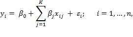
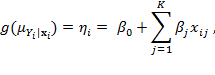
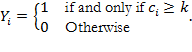
 . The former is referred to as the probit link function and the latter as the logit link function. The probit link function does not have a direct interpretation, while the logit is directly interpretable as we discuss below.[19]
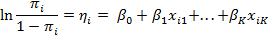
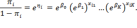
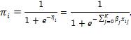
 Table 10.2 reports the logistic regression results of this poverty profile for West Java in 2007. Columns two to five report the estimated regression parameters along with their standard errors, t ratios, and significance levels at 5%[20]. Apart from being Muslim, all other determinants are significant at the 5% level and show the expected signs. For a given household, the log of the odds of being multidimensionally poor decreases with the education of the household head and with an urban location and increases with the presence of a female household head and with household size. The odds ratio for years of education of the household head indicates that an increase of one year of education decreases the odds of being multidimensionally poor by 49%, ceteris paribus, whereas having a female household head increases the odds of being multidimensionally poor by 28%, ceteris paribus.[21] Similarly, the odds of a household of being multidimensionally poor decrease by 57% for households living in urban areas, ceteris paribus, and increase by 10% for each additional household member. Figure 10.1 shows the odds model for urban and rural areas as a function of the education of the household head, holding constant the gender status of the household head (female), assuming five household members (average), and being Muslim. The logistic curves show a decrease in the probability of a household being multidimensionally poor as the education of the household head improves. These probabilities are lower for households living in urban areas compared to rural ones.
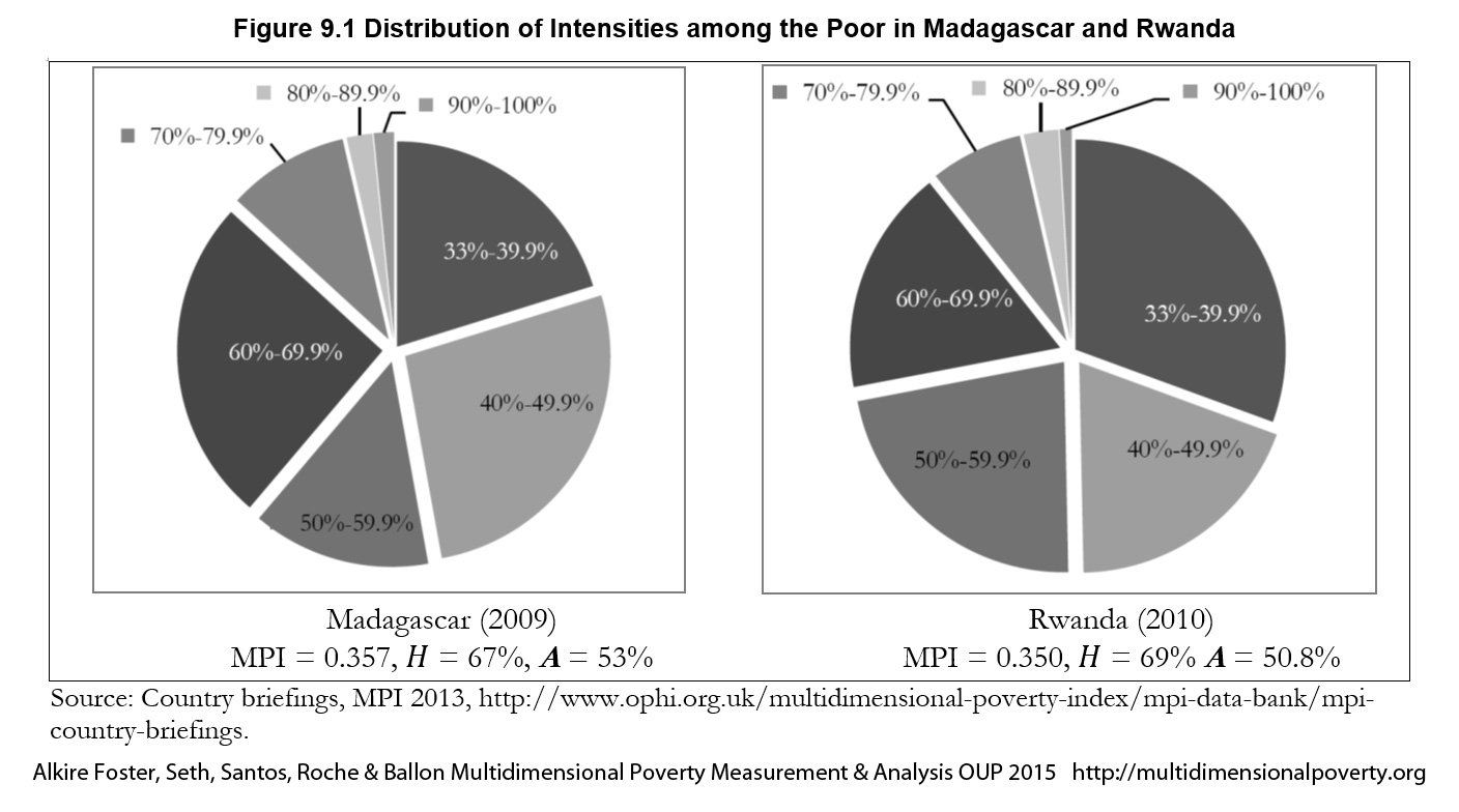

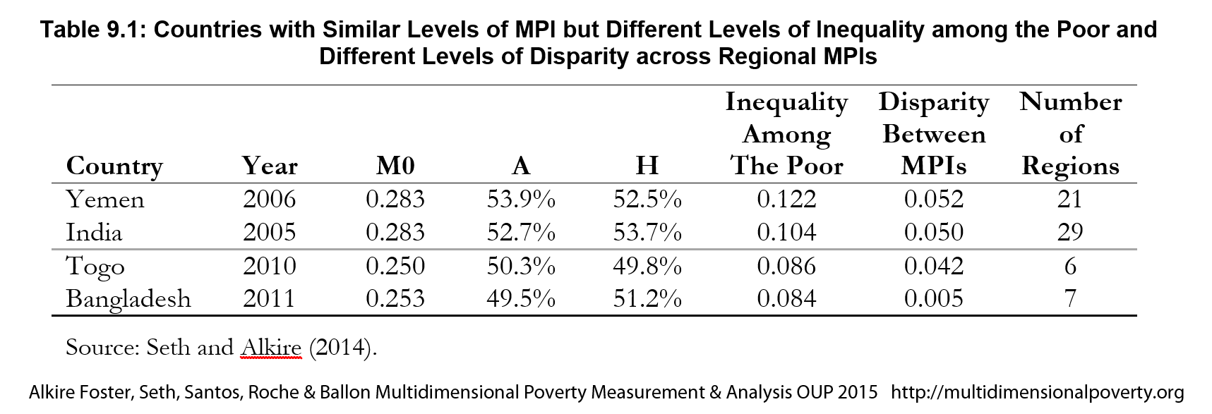
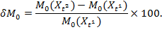
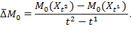
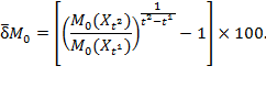
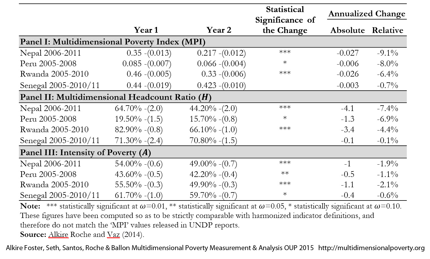
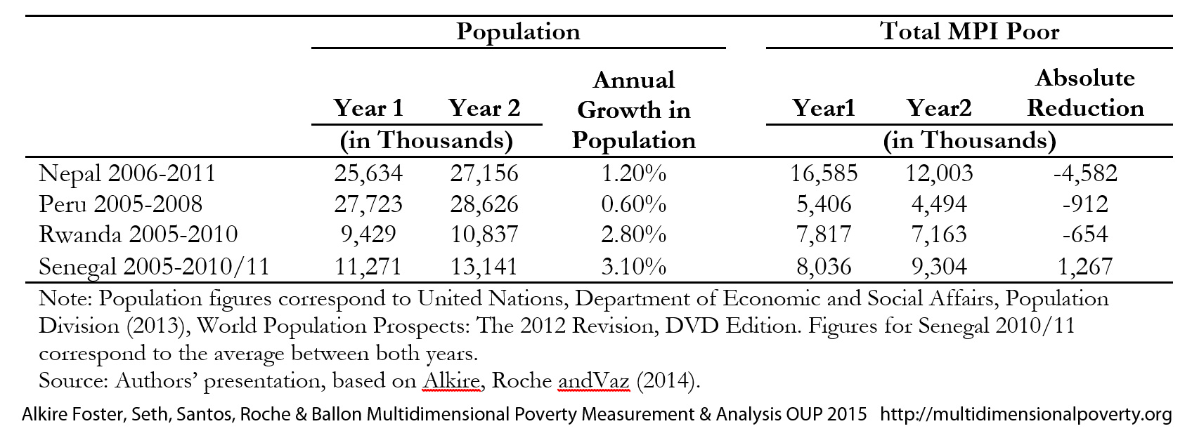
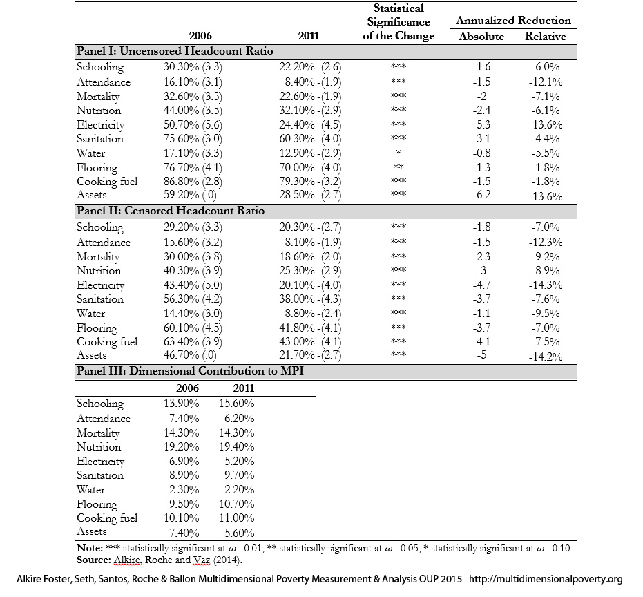
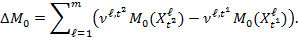
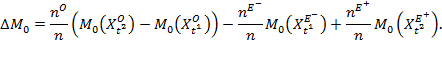
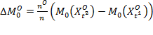 is due to the change in the intensity of those who remain poor in both periods—the ongoing poor—weighted by the size of this dynamic subgroup. The second component
 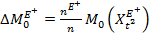 is due to the population-weighted change in the intensity of those who enter poverty. Together

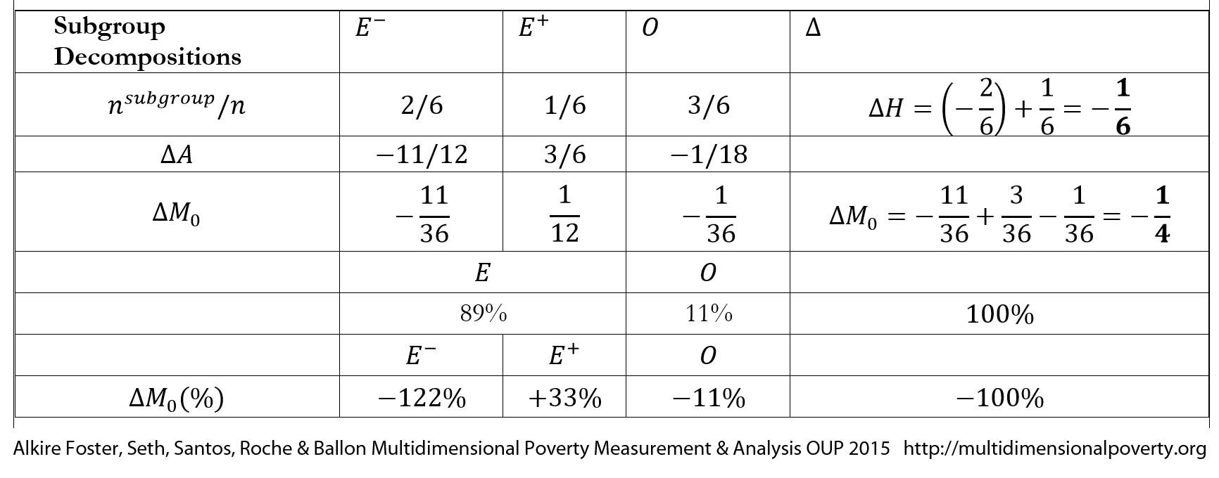
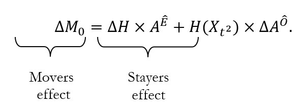
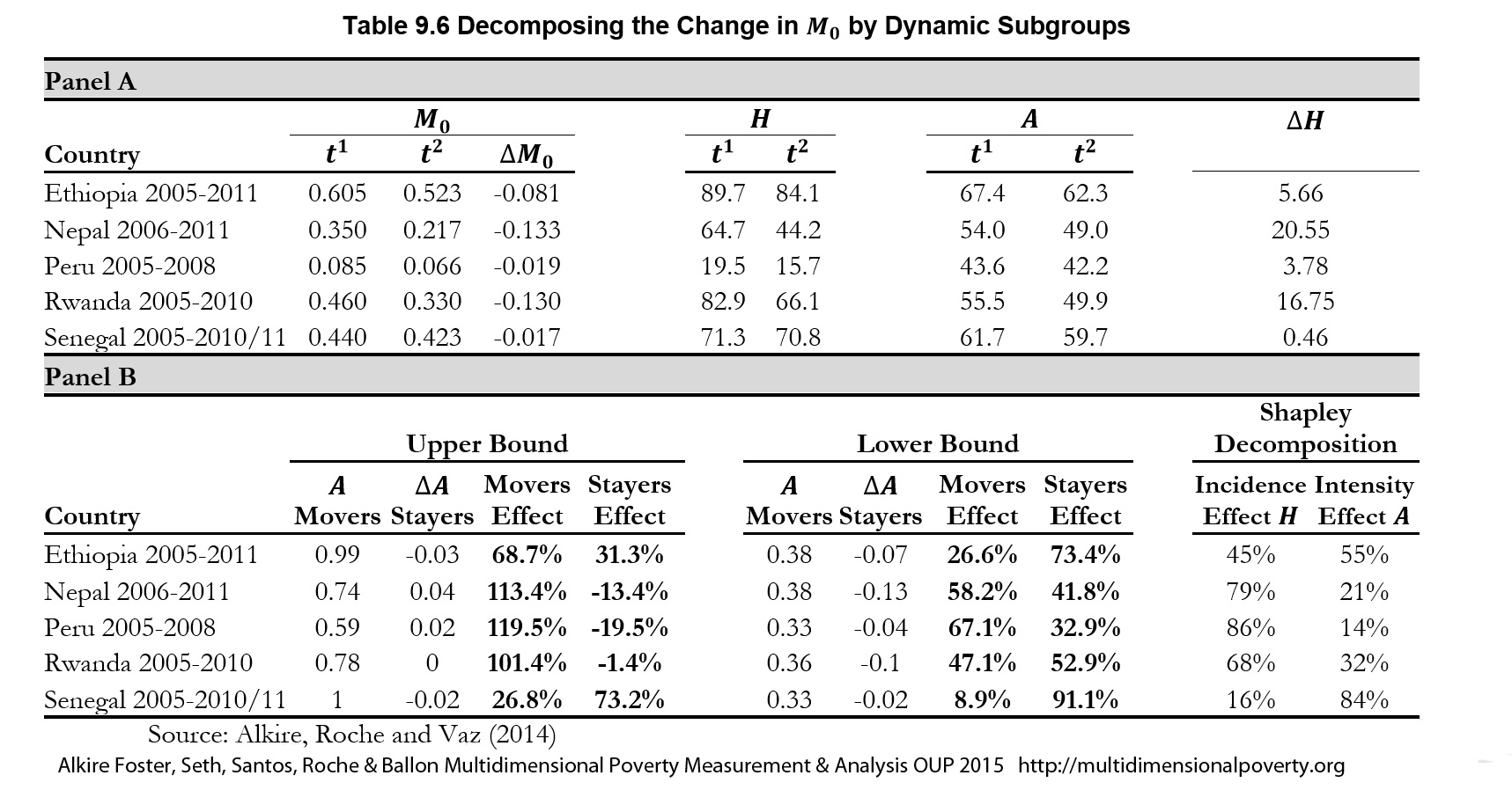
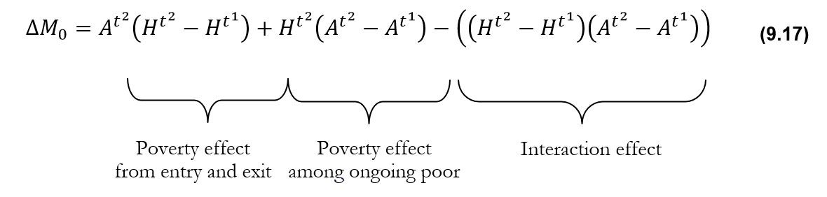
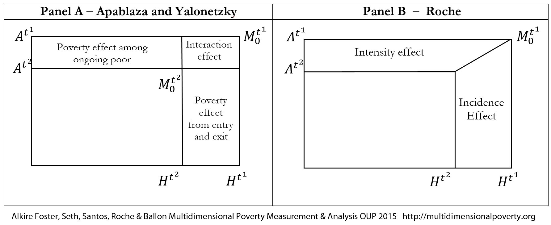
 , and calls this the ‘incidence effect’. He takes the other group as comprising the average headcount ratio between the two periods, and their change in intensity as the simple difference in intensities across the periods
  and describes this as the ‘intensity effect’.
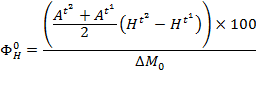
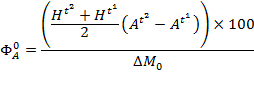
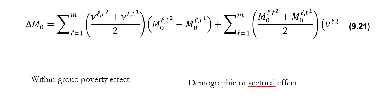
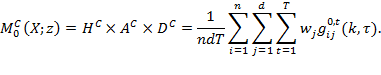
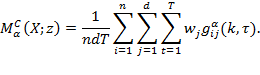
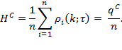
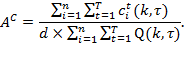
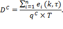
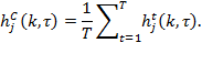
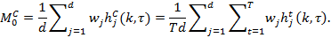
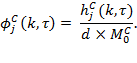
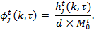
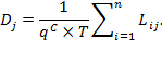
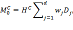
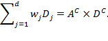


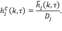
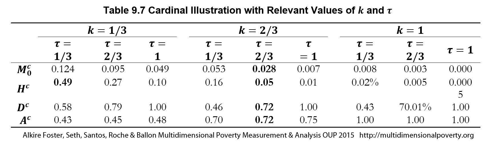
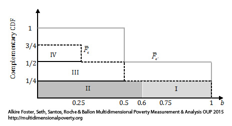
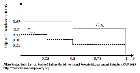
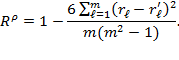
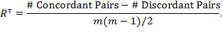

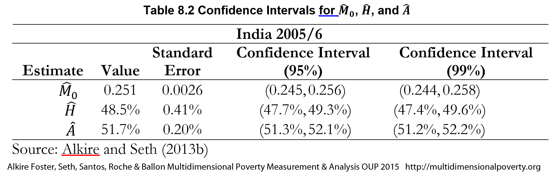
 . Note that, as we have assumed independent samples, the covariance between the two Adjusted Headcount Ratios is zero. Hence, the standard error of
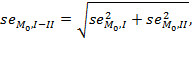
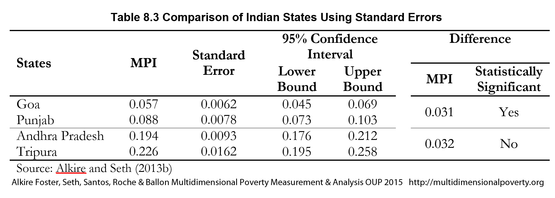
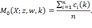
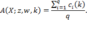
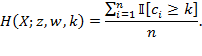
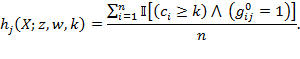
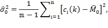
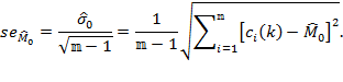
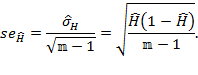
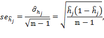
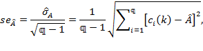
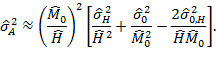
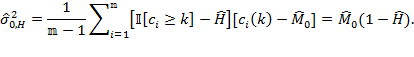
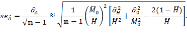
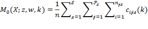
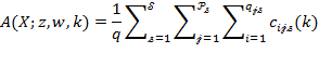
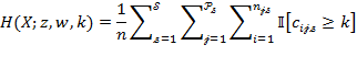
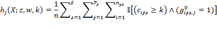
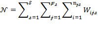
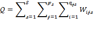
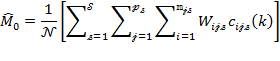
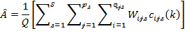
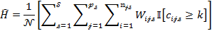
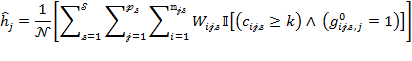
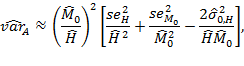
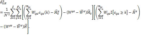
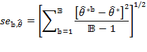

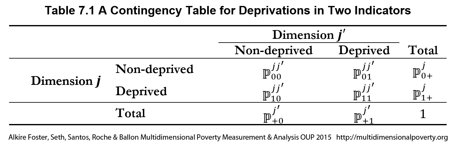
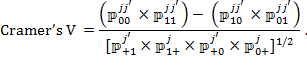
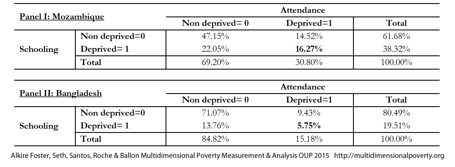
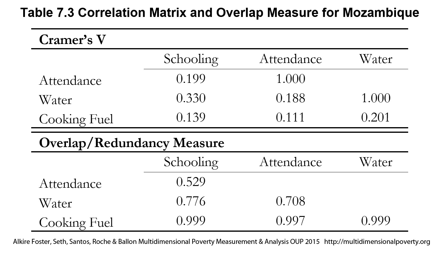
 ) for each person and indicator. The normalized gap is the difference between the deprivation cutoff and the poor person’s achievement for each indicator, divided by its deprivation cutoff. If a person’s achievement does not fall short of the deprivation cutoff, the normalized gap is zero. The average poverty gap is the mean of poor people’s weighted normalized deprivation gaps in those dimensions in which poor people are deprived and is one of the partial indices. This depth of multidimensional poverty is denoted by
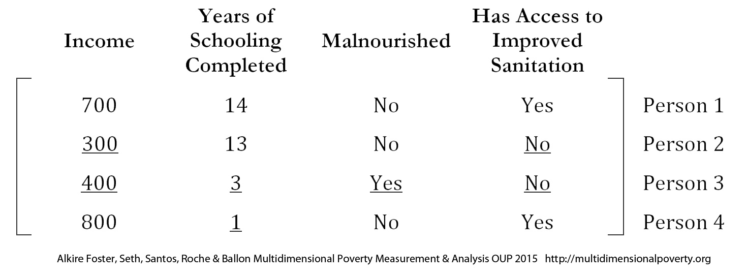
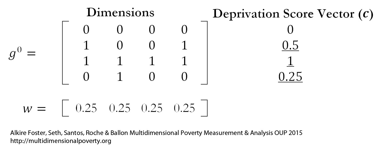

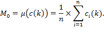
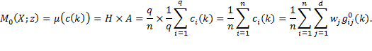
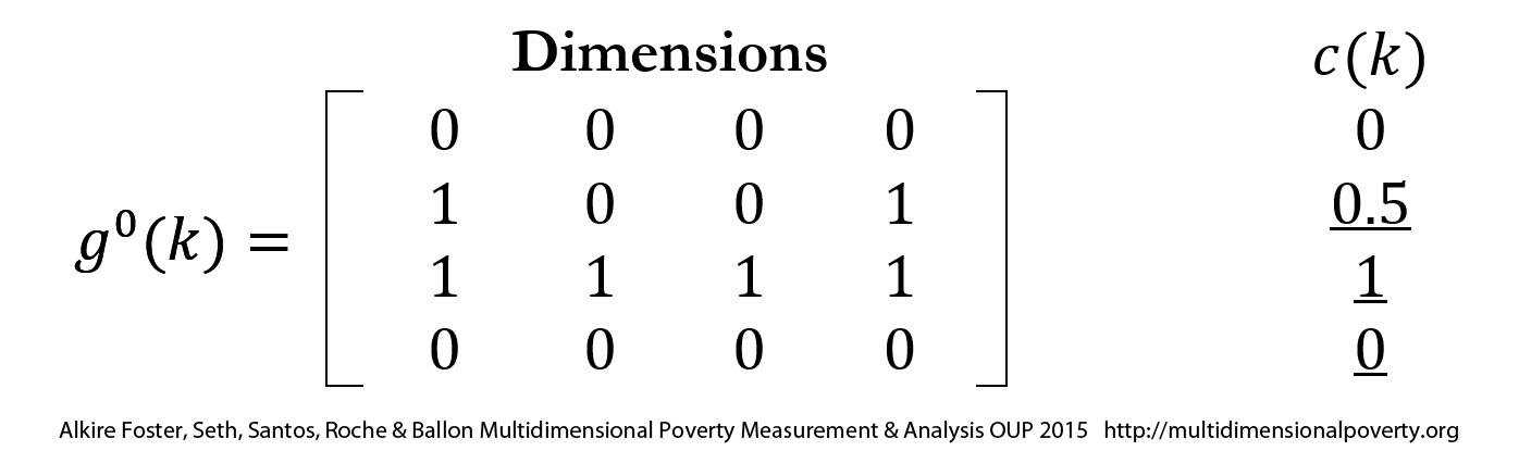
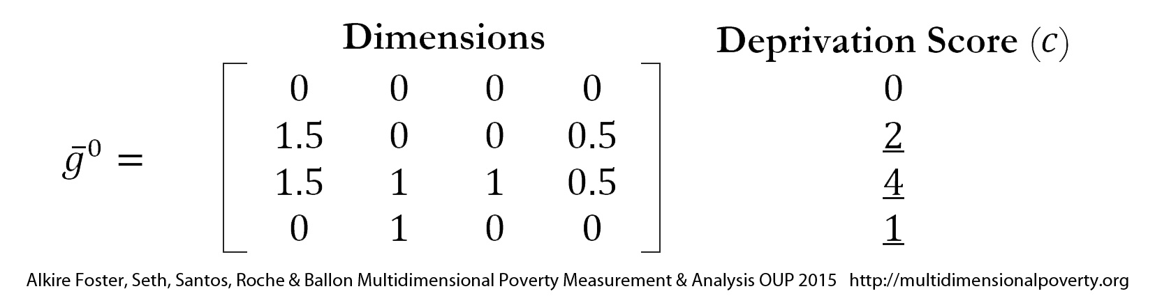
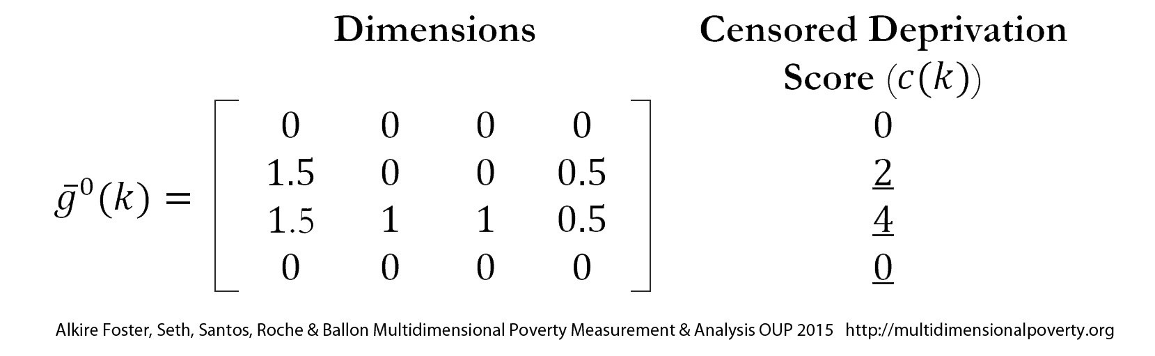
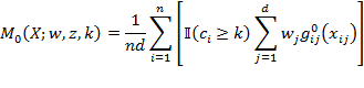

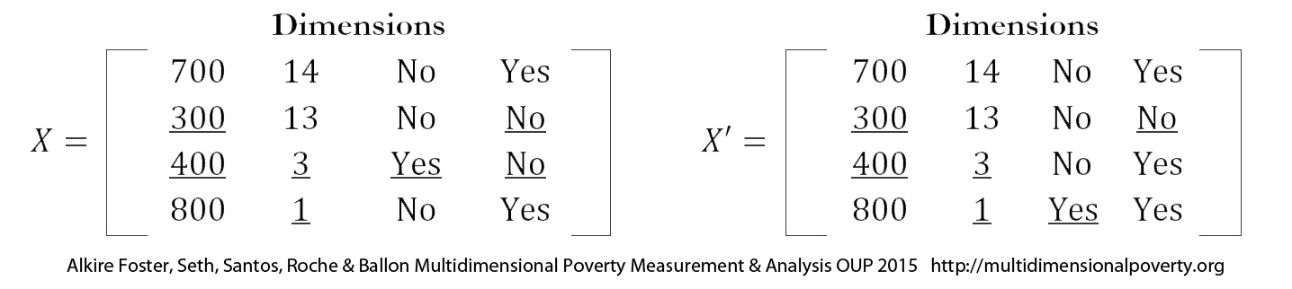

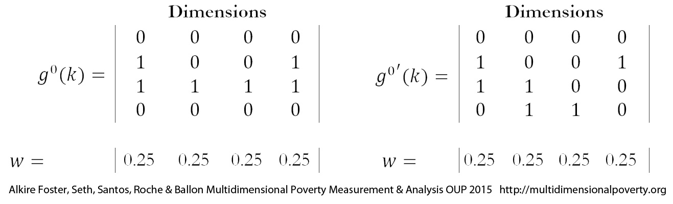
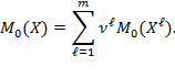
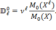
 )
)
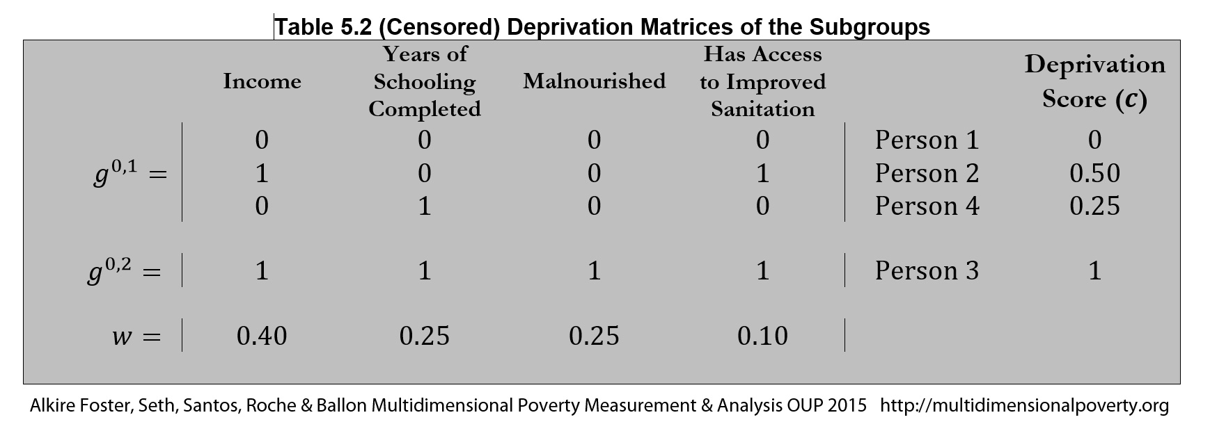

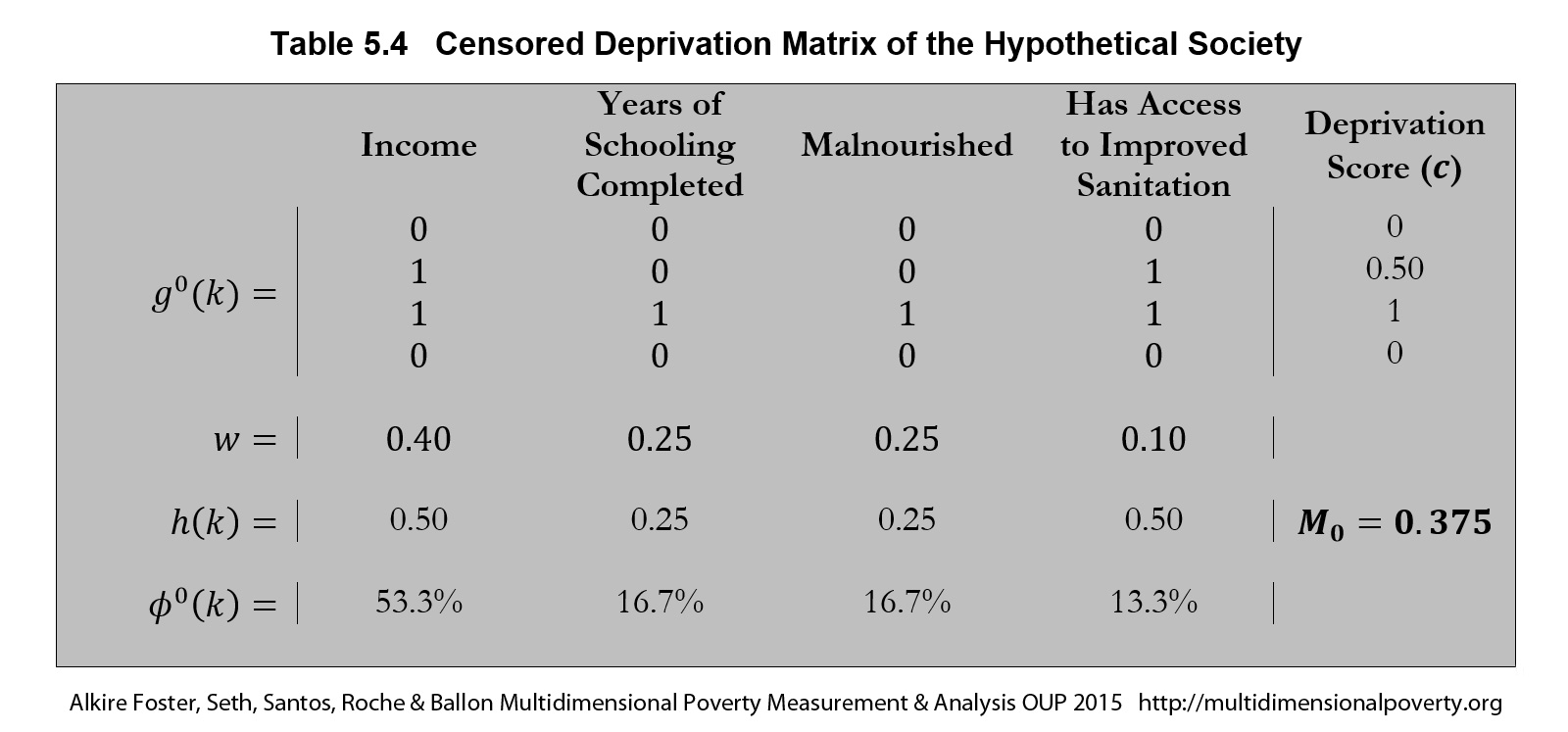


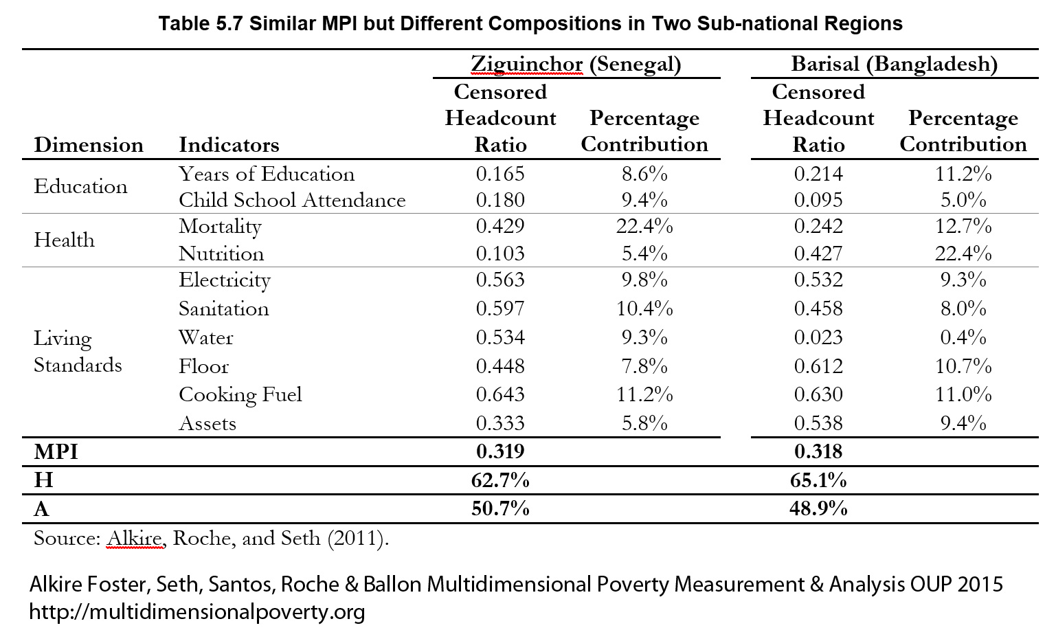
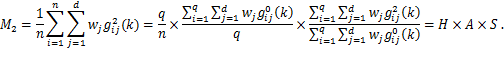
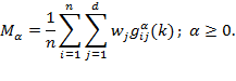
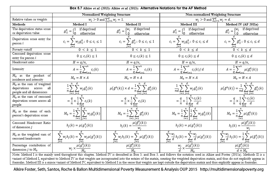

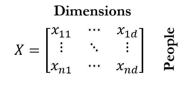
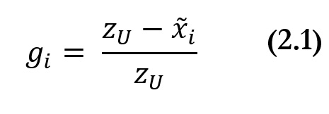
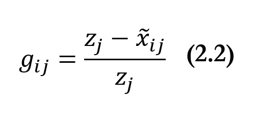
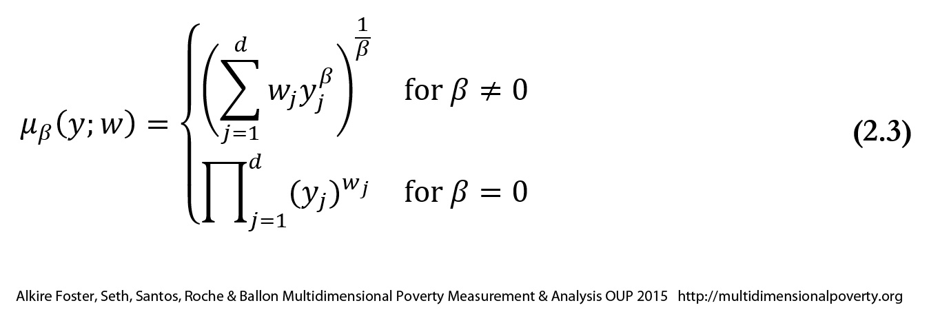
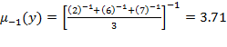 . The following graph depicts the values of the
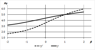
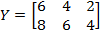 . Consider
  . Then
 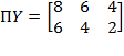 . Thus, the rows of
  . Then
  . Note that the second and the third columns have swapped their positions. The first column did not change its position because the first diagonal element in
  . Then
  . Each element in the first column has been halved and each element in the third column has been doubled. However, the second column did not change because the corresponding element of
  . Then
  . The bistochastic matrix equalizes the achievements across its elements.
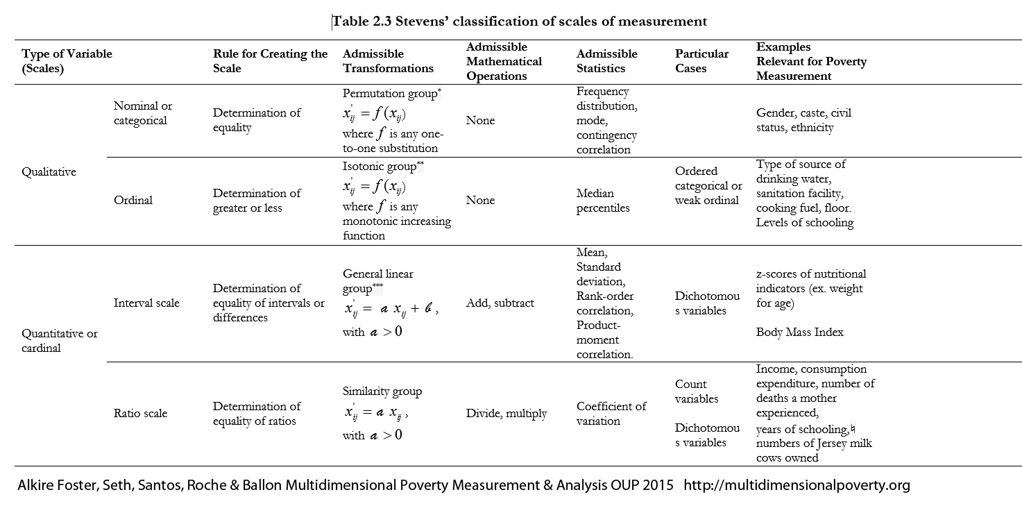
 and the permutation matrix is
 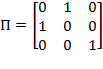 . Then:
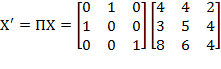
 . Note that the first and the second person (rows) in matrix
  . Note that the population sizes in these societies are different. In order to make them comparable, we replicate
  and
and  . By replication invariance, we know that
  to obtain
 . Similarly, vector
  , then by poverty focus,
  , then by the deprivation focus principle,
  and the deprivation cutoff vector is
  , and
, and  , then by the monotonicity principle,
  , then by dimensional monotonicity,
  , where the achievements are distributed equally across the two poor persons so that
  The transfer principle requires that
  . Suppose
  is obtained from
  by switching the achievements between the two poor persons in the third dimension. Clearly, an association-decreasing rearrangement has taken place between the two poor persons in
  is obtained from
 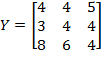 by switching the achievements between the two poor persons in the first dimension. Again, certainly an association-increasing rearrangement has taken place, but if we look at the achievements in the deprived dimensions of the two poor persons, they appear to be permutations of each other and thus overall poverty should not change. In order to make the transformations relevant in this situation, we need to ensure that the association-decreasing rearrangements occur only among the deprived dimensions of the poor. Thus, there is a need to define a new set of properties that is compatible with the deprivation-focus property, which can be done by defining the properties in terms of the censored achievement matrices. In this book, we define an additional set of new rearrangement properties by defining a transformation called association-decreasing deprivation rearrangement among the poor. Let
 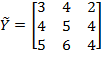 . Now, suppose
 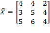 which is clearly not a permutation of
 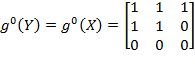 . A dimensional rearrangement among the poor is an association-decreasing rearrangement among the poor (in achievements) that is simultaneously an association-decreasing rearrangement in deprivations. In other words, the initial deprivation vectors (and achievement vectors) are ranked by vector dominance, while the final deprivation vectors (and achievement vectors) are not. The extra condition ensures that the person with a lower level of achievements is actually deprived in some dimensions in which the other person is not and that, through the rearrangement, one or more of these deprivations (but not all) are traded for non-deprived levels. More formally, let
  with population size