Multidimensional Poverty Measurement & Analysis

7 Data and Analysis

Chapter 6 transitioned from considerations about selecting a measurement methodology (Chapters 3–5), to issues met in implementing real-world measures that undergird and reinforce policies to fight poverty. It mentioned in passing the desiderata criteria that indicators be ‘technically solid’—a criterion that entails rigorous consideration of properties and also of empirical techniques. To take this forward, we now switch focus to emphasize the practice of empirical poverty measurement. In particular, this chapter introduces empirical issues that are distinctive to counting-based multidimensional poverty methodologies. Novel issues include the requirement that indicators accurately reflect deprivations at the individual level—not just on average—and that all indicators be transformed to reflect deprivations in the chosen unit of identification (person, household).

This chapter is not exhaustive. It presumes readers have a sound understanding of household survey data and micro-economic analysis, and also of various assessments of indicator validity. It supplements a presumed solid foundation with new elements that pertain to multidimensional poverty measurement design and analysis in particular. [1] A more extensive and detailed version is available at www.multidimensionalpoverty.org.

Section 7.1 introduces very briefly the different types of data sources available, namely, censuses, administrative records, and household surveys. Section 7.2 discusses issues to be considered when selecting the indicators to include in a multidimensional poverty measure. Finally, section 7.3 presents some basic descriptive analytical tools that can prove helpful in exploring the relationships between different indicators and informing the process of the measure design. Box 7.1 discusses the different fronts on which data collection should be improved in the near future in order to permit the design of better poverty measures.

7.1 Data for Multidimensional Poverty Measurement

As stated in Chapter 1, the initial step in poverty measurement, even prior to identification, is to select the space of analysis (resources, capabilities, utility) and the purpose of the measure to be constructed. The choice of space, as well as the feasible options for measurement design, will necessarily be shaped by data availability. We briefly review the main types of data used for multidimensional measurement and considerations of when to use each.

Multidimensional poverty is measured using micro data. By micro data we mean the unit-level data containing responses that each unit of analysis (such as person or household) provided. This contrasts with macro data, or aggregate indicators or marginal measures such as the mortality rate, literacy rate, mean household income, or the enrolment ratio, which summarize the achievements of a society. The three most common micro data sources are censuses, household surveys, and administrative records—also called register data. New relevant data sources such as mobile telephony and satellite imagery are rising sharply, and will deeply enrich future multidimensional poverty analyses.

A census is an enumeration of all households in a well-defined territory at a given point in time (Mather 2007). National censuses are typically conducted every five to ten years, and contain information on a strictly limited number of variables: demographic variables, such as nationality, age, gender, marital status, place of birth, location, ethnicity or religion, and language; social variables, such as literacy, educational attainment, and housing conditions; and economic variables, such as activity condition and employment (UNSD 2008; cf. United Nations 2008: 112–113, Table 1). Special censuses may be implemented for targeting and monitoring certain programmes, again using a few simple variables.

Censuses provide information with negligible sampling error (the whole population is considered) at highly disaggregated levels (municipalities–neighbourhoods). Census variables are used in the construction of multidimensional poverty maps using (and were previously used in the UBN tradition). And census data is essential for multidimensional measures that target individuals or households. The disadvantages of censuses are that (a) they have low frequency, (b) they offer information on a small set of indicators, and (c) micro data may not be available to researchers.

Administrative data refers to information typically collected by a government department or agency primarily for administrative purposes (birth registration, customs, administration of a social benefit, etc.). One prominent example is population registers constructed through a civil registration system (United Nations 2001). Population registers consist of an inventory of each member of the resident population of a country augmented continuously by information on vital events (births, deaths, adoptions, marriages, divorces, among others) (UNSD 2001). Other examples are tax, education, police, and health records.

Some advantages of using administrative datasets are that (a) they typically cover virtually 100% of the population of interest in a continuous form, (b) there are no added data collection costs, (c) there is data for individuals who might not normally respond to surveys, (d) when linked to other unit-level data sources, administrative data can produce a powerful resource for multidimensional poverty. However, there are also some disadvantages: (a) the information collected in administrative records is limited and may not match the research purpose, (b) any changes in data collection procedures or definitions may prevent comparability over time, (c) serious data quality issues may compromise accuracy, (d) metadata is usually not available,[2] (e) access to administrative (micro) data varies by country, and (f) linking data sources is rarely straightforward.

Household surveys are the most commonly used data source to study poverty. These collect on a sample or subset of the population. The sample may be representative of the population of interest, which can be the total population of a country or of a particular region or children under 15, or some other group.

The respondents for the survey are selected from what is called a ‘frame’ or list, which is usually obtained from the most recent census and is typically a list of households. Different sampling methods such as simple random sampling and complex multi-stage sampling are used in order for the sample to be representative of the population. Deaton (1997) offers a valuable introduction to each method.[3]

Household surveys were collected as early as the eigthteenth century in England (Stigler 1954). After World War II household surveys expanded internationally with India being a pioneer. Since the 1970s, several international programmes have promoted and supported the collection of household survey data in developing countries. These include the World Fertility Surveys, which were introduced in the 1970s and became the Demographic and Health Surveys (DHS) in 1984, and the World Bank Living Standards Measurement (LSMS) survey programme, ongoing since 1980 (Grosh and Glewwe 2000: 6). In 1995, the United Nations Children’s Fund (UNICEF) began its Multiple Indicators Cluster Surveys (MICS), and in 2000 the World Bank launched the Core Welfare Indicator Questionnaire (CWIQ). The World Bank also intensively supported the development and widespread fielding of household budget surveys and income and expenditure surveys that are used for income and consumption poverty measures and may contain other topics. Multidimensional poverty measures typically rely on multi-topic household surveys, which collect information with one survey instrument using a sample frame that has been defined to capture a diverse set of topics.[4]

7.2 Issues in Indicator Design

All data sources, however rich, impose constraints on a poverty measurement and analysis exercise. These are navigated via a number of important decisions that are made when designing a multidimensional poverty measure and choosing its component indicators. The following subsections address the ‘new’ empirical considerations that are relevant both in designing new surveys for multidimensional poverty and in implementing measures using existing data.

7.2.1 Unit-level Indicator Accuracy

A first essential and distinctive criterion for counting-based multidimensional poverty measures is that each indicator must be a relatively accurate reflection of the achievements enjoyed by each unit of identification across the relevant period and not simply the achievements enjoyed ‘on average’ by some group, as we will clarify in this section.

The unit of identification refers to the entity who is identified as poor or non-poor, (determination of the poverty status)—usually the individual or the household. In the literature of poverty measurement, this is typically referred to as the unit of analysis. However, the term unit of identification is more accurate because the identification may take place at a more aggregated level, but the analysis can still be performed at a more disaggregated level. For example, if the unit of identification is the household, analyses can still generate the percentage of the population who are poor.

Household surveys are usually designed to create indicators that are representative of the achievements and/or distributions of some population subgroups, such as states or ethnic groups, at the time of the survey. For example, there are indicators typically collected which have short reference periods in order to increase indicator precision, and are judged to be accurate ‘on average’ (Deaton and Kozel 2005). Prominent examples include consumption in the last seven days, illness in the last two weeks, and time use in the past twenty-four hours. The assumption is that people with unusually high consumption/health problems in the reference period will balance others with unusually low values, with the average (and in some cases, the distribution) being assumed to be accurate across the representative unit at the level of the single indicator. However achievements may not be accurate at the individual level. For example, if the last seven days’ consumption included a family wedding, if the respondent had a rare and brief bout of the flu in the past fortnight, or if the last twenty-four hours was a major public holiday, then a person’s response will not provide a good indication of his or her average consumption, morbidity, or time use over the past year. In contrast, indicators used for targeting people or households are always required to be accurate at the individual level.

Multidimensional measures require the joint distribution of deprivations to be accurate on average. This is straightforward to achieve if, as in the case of targeting, each indicator accurately identifies each person’s deprivations, and so the deprivation scores, which reflect joint deprivations and will determine whether or not the person is identified as poor, are similarly accurate at the individual level. Selected indicators ideally balance indicator precision and unit-level accuracy in order to justify the assumption that responses reflect individual or household achievement or deprivation status during the relevant period. A related requirement, which occurs when multidimensional poverty measures (and, incidentally, other measures) are used to track trends in poverty over time, is that the indicators should ideally reflect individual achievement levels across the relevant period so that the comparisons are not unduly distorted by seasonal effects or short-term shocks.

Many indicators are relatively unproblematic in this regard. Indicators such as child vaccination, completed years of schooling, child mortality, housing materials, chronic disability, or long-term unemployment, for example, are likely to reflect individual or household achievements accurately. Moreover, a non-union identification strategy in the poverty cutoff can partially, as we discussed in Chapter 6, ‘clean’ data of errors.

That being said, in the case of other indicators, particularly those with short reference periods, the ideal may be more difficult to obtain. In practice, when collecting primary data, the unit-level accuracy issue should be considered when creating the questionnaire. When using secondary data, unit-level accuracy may guide the choice between different indicators, when such an option exists.

7.2.2 Indicator Transformation to Match Unit of Identification

Alkire-Foster multidimensional poverty measures reflect the joint distribution of deprivations for a given unit of identification. While the advantages of this and related approaches have been much discussed in Chapter 3, its empirical implementation actually requires novel techniques. In particular, relevant data may be available for individuals, for the household, and, perhaps, also at the community level. But it is necessary to transform all indicators such that they reflect deprivations of just one (the chosen) unit of identification. Consideration of the unit-level profile of joint deprivations leads to its identification as poor or non-poor (based on the poverty cutoff and deprivation score) and hence to the inclusion or censoring of its deprivations in the resultant multidimensional poverty measure.

To begin with an elementary case, consider a child poverty measure covering children aged six to twelve. Suppose that there are data on children’s education, health, and nutrition; household-level data on income and housing; and village-level data on the quality of primary school facilities. In the achievement matrix, each child will naturally have their own achievement levels in health, education, and nutrition. All children from the same household may take the household’s achievements in income and housing. And all school-going children in the same village may have the same achievements in quality of school facilities. The proposed transformations of household- and community-level data imply the assumption that the household- and community-level variables affect each child in the same way—which may require justification. The deprivation cutoffs for each indicator will be applied to this matrix, and each child will be identified as deprived or non-deprived in each indicator and, subsequently, as poor or non-poor, based on their weighted deprivation score. Thus each child’s deprivation profile will draw on data from individual-, household-, and community-level sources. In this way, household- and community-level indicators can be appropriately ‘transformed’ so they inform the deprivation profile of each child. But many cases are not so simple. The next section will set out how to proceed in those cases.

7.2.3 The Unit of Identification and Applicable Population

We begin with an important definition. The applicable population of a certain achievement refers to the group of people for which such an achievement is relevant; namely, it can be measured and has been effectively measured, in this case, to inform poverty measurement. Note that both conditions need to hold for the population group to be applicable.[5] In some cases, the achievement is conceptually applicable to the whole population (with appropriate adjustments in the levels considered adequate by age group or gender), but, despite this, data is typically not collected at the individual level. An example of this is the case of anthropometric indicators (nutritional indicators). While there are anthropometric indicators for all age groups and genders, these are often collected only for children under 5 years of age and for women of reproductive age. Thus for those anthropometric indicators, the remaining population groups are non-applicable because of data constraints. In other cases, the achievement is conceptually inapplicable to certain groups of the population, as in the case of income earned by infants. In either of the two cases, the existence of non-applicable populations poses a problem to be resolved when constructing a poverty measure, if that measure is to reflect their poverty also.

The choice of the unit of identification and the treatment of non-applicable populations are often constrained by data availability. In many cases, the ideal unit of identification would be the individual; another commonly used unit is the household. In this case, the household is judged to be poor or not, and all its members are then identified as poor. ‘The standard apparatus of welfare economics and welfare measurement concerns the wellbeing of individuals. Nevertheless, a good deal of data have to be gathered from households…’ (Deaton 1997: 23). Both units have advantages, as discussed in Chapter 6.

If the unit of identification of the poor is the individual, then all the considered achievements need to be available at the individual level, and thus all the achievements need to be applicable to the whole population for which the poverty measure is defined. If the unit of identification is the household, then one data point on common achievements like housing and heating may be applied to all household members. But not all the considered achievements are equally applicable to the whole population—income being a case in point (see below, this section). In these cases, certain (explicit) assumptions need to be made regarding the sharing and impact of the achievements of certain household members with respect to the others. Other achievements are individual—like health status or educational level—although they may affect household members also.

Strictly speaking, few household-level indicators are applicable to each household member. Most vary by age and some by gender. Housing conditions are an example of indicators that satisfy the ‘universality’ of applicable population. Any person, regardless of age or gender needs a clean source of drinking water; adequate flooring, walls, and roof; clean cooking fuel; and adequate sanitation, for example. Such dwelling conditions are jointly consumed by the household. Household surveys collect information on the dwelling conditions, and for poverty analysis it is then assumed that all members equally share them—although this may or may not be accurate.

Another universally relevant and applicable indicator for all people, now at the individual level, is nutritional status. In this case, one will need to combine at least two indicators: one for the nutritional status of children under 5 years of age (which can be weight-for-age, weight-for-height, or height-for-weight) and another for the nutritional status of adults, typically the Body Mass Index (BMI).[6]

Food consumption is another universal indicator. Although nutritional requirements vary significantly by age and gender, it may be possible to define the relevant consumption range for each type of individual.[7] However, data availability usually poses a limitation: ‘Household surveys nearly always collect data on household consumption (or purchases), not on individual consumption, and so cannot give us direct information about who gets what’ (Deaton 1997: 205). Thus, even though conceptually food is a private consumption good, applicable to each member of the population, in practice, it is often assumed that total consumption is distributed within the household in proportion to the nutritional requirements of each member. This assumption may or may not be accurate.

Income is not a universal indicator, as it is inapplicable to people who lack income from non-labour sources like financial assets and do not earn an income (for example, babies and children, housewives, non-working students, and some elderly members) or are unemployed. Standard income poverty measures aggregate all forms of household members’ income (labour or capital) and divide by the total household size (including the members who do not earn an income) to obtain the household per capita income. Equivalence scales may be applied to obtain the household adult equivalent income. The per capita or adult equivalent income is compared to the poverty line, and the household is identified as poor or not and thus all its members. Here, as in the case of consumption, assumptions regarding equal or proportional sharing have been made.

Some other relevant indicators for poverty measurement which are inapplicable for certain groups include child vaccination (adults and children older than the relevant age group do not qualify), child mortality (people who have not had children do not qualify), and employment status. Even education as measured, for example, by years of schooling is not universally applicable, as children below the official mandatory age for starting school do not qualify.

Given that some achievements relevant for poverty measurement are either conceptually or empirically applicable only for certain population groups, the selection and definitions of indicators may take one of the following three options, depending on the purpose of the measure. They may also work as complement measures. The options are :[8]

(a) To restrict consideration to universally applicable achievements

(b) To construct group-specific poverty measures

(c) To combine achievements that are not universally applicable and test assumptions regarding intra-household distribution and/or impact.

(a) Universal measures

One option is to include ‘universal’ achievements, that is, achievements which are applicable to the whole population. This approach narrows the set of possible indicators, although it will include housing, consumption, nutrition, and access to services, if data permit.

(b) Group-specific measures

A second option is to construct different poverty measures for each relevant group, such as child poverty measures, or measures of female or elder poverty. This is an attractive option and suited to group-based policies such as for children or women or elders.

However, three issues need to be considered. First, discriminating by groups may lessen but not eliminate applicability issues. For example, the relevant nutritional indicators change at the age of five, whereas schooling becomes mandatory typically at the age of six or seven, and vaccination ages vary. Thus no group is perfectly homogeneous and indicators may need to be adjusted within population subgroups. Second, it may be critically important to have detailed poverty analyses by population subgroups and these may inform group-based policies profoundly. Yet ‘general’ measures may also be required to track national poverty or to target households. Finally, using unlinked poverty measures for different population subgroups may miss the overlaps of disadvantaged groups and fail to fully exploit possible synergies in policy design.

(c) Combined measures

The third option is to use achievements drawn from a subset of household members (or other unit of identification), and make explicit assumptions about the distribution of such achievements and potential positive or negative intra-household externalities.

This has been the route taken when constructing the global Multidimensional Poverty Index (MPI) (Alkire and Santos 2010, 2014). Assume for example that one wants to include nutrition but information was only collected for children under five and women of reproductive age. Given these data constraints, a household nutrition deprivation indicator might be defined as ‘having at least one child or woman undernourished’. Hence, any household member is considered deprived in nutrition if—despite being well nourished herself—any child or woman is undernourished in her household. Similarly, if one wants to include an indicator of child mortality in the poverty measure, one way to proceed is to consider all household members as deprived if even one child in the household has died. Analogously, one can consider all household members as deprived if there is at least a child of school age who is not attending school. In all of the three examples above there is an obvious assumption of a negative intra-household externality produced by the presence of an undernourished person, the experience of a child’s death, or a child being out of school. Indicators based on the assumption of a positive intra-household externality are also possible. For example, in the global MPI all household members are considered non-deprived if at least one person has five years of schooling, assuming that there is interaction and mutual sharing of cognitive skills within the household as suggested by Basu and Foster (1998).

Two practical situations must be addressed in order to compute combined measures. First, there are households where not even one person qualifies for the achievement under consideration. For example, a household may not have any children in the relevant age bracket. What indicator is used to define deprivation in these households? There is no perfect procedure. Dropping these households from the sample would bias the estimates, as the inapplicability of a certain achievement to a particular population subgroup is not a random issue and households without that population subgroup would be systematically excluded.[9] Dropping any indicator for which no applicable person is present in a household and reweighting the remaining indicators would violate dimensional breakdown and compromise comparability across people. A viable option is to consider all households lacking the relevant data as non-deprived (or deprived) in that particular indicator, then scrutinize this assumption. For example, a household with no children of school age cannot be deprived in child school attendance, so they could be considered non-deprived in this indicator.

A second situation occurs when the survey has not collected information from all applicable members. The example of nutrition above illustrated this case. Nutrition is applicable to all household members, yet some surveys only collect information on children and women in reproductive age, for example. So households that do not have children or women in reproductive age lack data altogether As above, all such households may be considered as non-deprived (or deprived) in that indicator. Clearly, considering them as non-deprived is a heroic assumption, as we simply do not know because information is not available. But it could be seen as a ‘conservative’ approach (in the same spirit of the ‘presumption of innocence’ principle in legal arenas), and will lead to a ‘lower bound’ poverty estimate. That is, it will offer the minimum possible estimate of the proportion of people in households with an undernourished member, which could be improved later.

Naturally the assumptions used in measurement design should be examined empirically as well as debated normatively. Special studies of omitted populations (such as the elderly), including qualitative studies, should be considered to enrich measurement design and analysis, and results should be compared with group-based results to cross-check conclusions.

7.2.4 Assessing Combined Measures

Most multidimensional poverty measures are ‘combined measures’, hence some assumptions are made to permit analysis. This section describes how to assess key assumptions. Two particular kinds of analysis may be especially relevant. The first is related to the household composition effect; the second is related to the prevalence of the indicators.

First, by including indicators referring to achievements that are specific to certain groups (such as school attendance), the composition of the household will affect the probability that the household will be identified as poor. Taken to the extreme, if all the indicators in the poverty measure refer to a deprivation that can only occur among children, then clearly households without children would never be identified as poor. Obviously, a balance regarding the relevant populations for the considered achievements is required. The potential effect of household composition need not prevent the inclusion of an indicator if its importance is normatively clear. For example, it may be the case that there is a national concern about child nutrition. Inclusion of such indicators can be made provided (a) not all of the indicators in the poverty measure refer only to a particular specific group (if so, then a group-specific poverty measure is a better alternative); (b) the specific group for which the achievement is relevant is big enough so that a known and significant proportion of households have at least one member for whom the achievement is relevant; and (c) an empirical assessment of the impact of household composition is performed to test the sensitivity of the measure to its specification.[10]

For example, Alkire and Santos (2014) present two assessments of the influence of household composition on the probability of being poor. The first are hypothesis tests of differences in means. In each country they test whether MPI-poor households have a significantly different average size, average number of children under 5, number of females, number of members 50 years and older, prevalence of female-headed households, and proportion of school-aged children, compared to non-poor households. The second analysis decomposes each country’s MPI by age and gender and compares the rankings, correlations, and the proportion of robust pairwise country comparisons across subgroup MPIs.

Regarding requirement (b), some deprivations are intrinsically important yet are either rare events or pertain to population subgroups that are very small, and thus the presence of a household member for whom the deprivation is relevant is quite unlikely. Under such circumstances, it is best to keep this indicator separate from the multidimensional poverty measure. Examples of such indicators vary by context but might include prevalence of a rare condition that affects pregnant women.

7.2.5 Handling Missing Values

The construction of household variables (for example), from data pertaining to a subset of household members described above is completely separate from the need to address missing values, to which we now turn.

Missing values are particular cases for which a variable that is collected by the survey is not available. For example, if there is a woman of reproductive age for whom the information on BMI should have been collected, given the survey design, but for whom this information is incidentally not available, that is a case of a missing value. Missing values require attention in all poverty measures; multidimensional poverty measures have the advantage of using fewer variables than many monetary measures, but the treatment of missing values also differs slightly.

There are essentially two ways of dealing with missing values. One is to drop that observation from the entire sample. That is, if the unit of identification is the household, households with a missing value in any indicator for a multidimensional measure are dropped from the sample.

The other option is to create a rule that may assign a value for the missing data, particularly in a combined measure in which, for example, data are missing only for some individuals for whom the indicator is applicable. For example, in the case of the global MPI, if at least one member has five or more years of education (although other members have missing values), the household was classified as non-deprived. If there was information on at least two-thirds of household members, each having less than five years of education, the household was classified as deprived; otherwise it was dropped from the sample (Alkire and Santos 2014).

If the observations with missing values systematically differ from those with observed values, the reduction in the sample leads to biased estimates. To assess whether the sample reduction creates biased estimates, the group with missing values is compared to the rest, using the indicators for which values are present for both groups. If the two groups are not (statistically) significantly different, then one may proceed with an estimation using the reduced sample. If they are (statistically) significantly different, then one may still use the reduced sample but should explicitly signal whether the poverty estimate is likely to be a ‘lower’ or an ‘upper’ bound, based on the results of the bias analysis (Alkire and Santos 2014).[11]

One might consider whether to use imputation to assign the observation with a missing value an estimated value of the indicator under consideration. This is commonly done in income poverty measurement, but further research is required before it is applied multidimensionally. Imputation techniques entail using the observations for which there is information to estimate a model with the achievement under consideration as the dependent variable against a set of explanatory variables. The estimated parameters are then used to predict the achievement for the cases with missing values, given their values in the explanatory variables. However, imputation techniques are not problem-free. First, the estimated model needs to be accurate. Second, in the case of multidimensional poverty measurement, the issue of missing values is multiplied because what is of interest is each person’s joint distribution of deprivations. This poses a significant challenge for imputation. One could specify a different model for each indicator. However, when that option is taken, it is likely to incur endogeneity problems. Moreover, this option is blind to varying profiles of joint deprivations. The more accurate route to take would be to specify a model that could predict a vector of deprivations. This imputation would also have to be performed such that it was accurate for each unit of identification, not merely on average. But this has not been done yet. Third, and connected to the previous section, it is also worth noting that imputation techniques cannot solve the problem of non-applicable populations as there are no observations that can be used to estimate a model. For example, one cannot impute the BMI of elderly people using a survey that collects BMI information only for women of reproductive age. As the field of multidimensional poverty measurement progresses, appropriate imputation techniques may be developed for this context.

7.3 Relationships among Indicators

Before implementing any measure empirically it is helpful to understand the variables that may be entered into the measure: by looking at univariate and bivariate statistics such as measures of central tendency, dispersion and association. In the presence of multiple dimensions it is helpful to view their joint distribution, to scrutinize the associations across dimensions and explore similarities or redundancies that may exist.[12] Such analysis may lead one to drop or re-weight an indicator, to combine some set of indicators into a subindex, or to adjust the categorization of indicators into dimensions. It can also inform the selection of indicators and their robustness checks, the setting of deprivation values, and the interpretation of results.

Statistical approaches are relevant for multidimensional poverty measures, but Chapter 6 argued, value judgements also constitute a fundamental prior element. Thus, information on relationships between indicators is used to improve rather than determine measurement design. For example, if indicators are very highly associated in a particular dataset, that is not sufficient grounds to mechanically drop either indicator; both may be retained for other reasons—for example if the sequence of their reduction over time differs, or if both are important in policy terms. So the normative decision may be to retain both indicators, with or without adjustments to their weights, but the analysis of redundancy will have clarified their justification and treatment.

The techniques commonly used to assess relationships between indicators include many of those already presented in section 3.4—that is, principle component analysis, multiple correspondence analysis, factor analysis, cluster analysis, and confirmatory structural equation models, as well as cross-tabulations and correlations. This section is limited to explaining the limitations of correlation analysis between deprivations and introducing a distinctive indicator of redundancy. Both of these draw on contingency tables presented in section 2.2.3. It is further limited in that we restrict information to the dichotomized deprivation matrix, using only uncensored or censored headcount ratios for each indicator.

7.3.1 Cross-Tabulations

As was mentioned earlier, cross-tabulations or contingency tables are a basic way to view the joint distribution between two dichotomous variables—which could be the uncensored or censored headcounts. We return to these to consider matters of correlation and redundancy. A two-way contingency table (Table 7.1) provides information on two kinds of matches:

: The percentage of people simultaneously not deprived in any two indicators and

: The percentage of people simumtaneously deprived in any two indicators and )

It also shows two kinds of mismatches:

: The percentage of people deprived in indicator but not in indicator

: The percentage of people deprived in indicator but not in indicator .

Finally, it shows the ‘marginal’ distributions as and so on. Note that two of these marginals will correspond to the uncensored or censored headcount ratios of the two indicators.

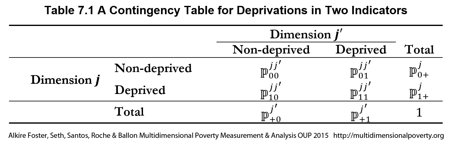
We show this familiar building block to remind readers that correlations between dichotomous variables (which generate the same coefficient as the Cramer’s V), draw on all elements of the cross-tab: the matches, the mismatches, and the marginal entries. In words, the correlation is the product of the matches minus the product of the mismatches, divided by the square root of the product of the marginals

(7.1)

 

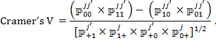
What is important to notice is that while the correlation is affected by the extent to which deprivations between variables match (which is key for redundancy), it is also affected by values of the headcount ratios and their difference. This, as we will show, somewhat dilutes the insights that correlations offer for redundancy, so that the correlation coefficients are best interpreted alongside the contingency table for each indicator pair. Similarly, PCA, MCA, and FA also use all elements of the cross-tab.

Instead of using the correlation (Cramer’s V) alone, we propose another measure of association, which has some attractive characteristics for a direct assessment of redundancy.[13] This measure shows the matches between deprivations as a proportion of the minimum of the marginal deprivation rates. If two deprviation measures are not independent, and if at least one of the headcount ratios is different from zero, then the measure of Redundancy or Overlap is defined as

(7.2)

That is, the measure of Redundancy displays the number of observations which have the same deprivation status in both variables, which reflects the joint distribution, as a proportion of the minimum of the two uncensored or censored headcount ratios. By using the ‘minimum’ of the uncensored or censored headcounts in the denominator we ensure that the maximum value of is 100%.

If takes the value of 80%, this shows that 80% of the people who are deprived in the indicator having the lower marginal headcount ratio are also deprived in the other indicator. Thus a high level of is a more direct signal that a further assessment of redundancy is required than a correlation measure might be.

An example will clarify and close this section.

1. Contingency Tables for Mozambique and Bangladesh

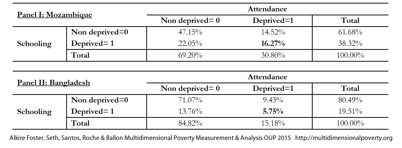
Consider the Contingency Tables in Panel I and II of Table 7.2, which draw on 2011 DHS surveys for each country. In Mozambique, 38% of the population are deprived in years of schooling and 31% in school attendance. Only 16% are deprived in both indicators. For Bangladesh, 20% and 15% are deprived in years of schooling and school attendance respectively, and 6% are deprived in both. How do we assess the association between these indicators? Consider first the correlation or Cramer’s V coefficients, computed using equation (7.1). Using the values in Table 7.2 it can be easily verified that the Cramer’s V between attendance and schooling is 0.199 for Mozambique and 0.196 for Bangladesh. They are quite similar. But when we compute the measure using equation (3.30), we find that 52.8% of possible matched deprivations overlap for Mozambique, but only 37.9% match for Bangladesh. focuses on the precise relationship of interest.

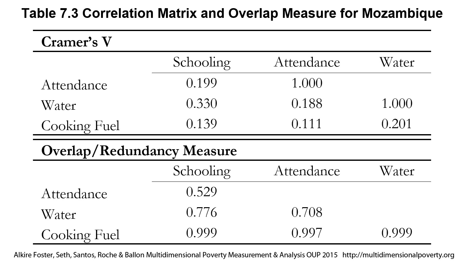
Table 7.3 gives the Cramer’s Vs (correlation coefficients) and the measures of overlap/redundancy for three pairs of indicators for Mozambique. The highest redundancy values correspond to those between cooking fuel and other indicators. These are exceedingly high and might suggest that cooking fuel is redundant in these datasets, unless it is retained for other normative reasons (sequencing, policy). Yet the Cramer’s Vs between for cooking fuel and other dimensions are not particularly high and would not show this—indeed the correlation between water and schooling is much higher. As explained above, the divergence between these two values reflects the different components of the cross-tab that they draw upon. Although correlations are often used, we consider the measure of overlap to provide clear and precise information that should be considered alongside other kinds of information in evaluating indicator redundancy.

Chapter 8 addresses robustness analysis and statistical inference, which are required to draw conclusions or guide policies based on estimated poverty measures.

Bibliography

Alkire, S. and Ballon, P. (2012). Understanding Association across Deprivation Indicators in Multidimensional Poverty. Paper presented at the Research Workshop on ‘Dynamic Comparison between Multidimensional Poverty and Monetary Poverty’. OPHI, University of Oxford.

Alkire, S. and Santos, M. E. (2010). ‘Acute Multidimensional Poverty: A New Index for Developing Countries’. OPHI Working Paper 38, Oxford University; also published as Human Development Research Paper 2010/11.

Alkire, S. and Santos, M. E. (2014). ‘Measuring Acute Poverty in the Developing World: Robustness and Scope of the Multidimensional Poverty Index’. World Development, 59: 251–274.

Basu, K. and Foster, J. (1998). ‘On Measuring Literacy’. Economic Journal, 108(451): 1733–1749.

Browning, M. (1992). ‘Children and Household Economic Behavior’. Journal of Economic Literature, 30(3): 1434–1475.

Deaton, A. (1997). The Analysis of Household Surveys. A Microeconometric Approach to Development Policy. John Hopkins University Press.

Deaton, A. and Kozel, V. (2005). ‘Data and Dogma: The Great Indian Poverty Debate’. World Bank Research Observer, 20(2): 177–199.

Deaton, A. and Muellbauer J. (1980). Economics and Consumer Behavior. Cambridge University Press.

Grosh, M. and Glewwe, P. (2000). Designing Household Survey Questionnaires for Developing Countries: Lessons from 15 Years of the Living Standard Measurement Study, vol. 1. The World Bank.

Hagenaars et al. (1994): Hagenaars, A., de Vos, K., and Zaidi, M. A. (1994). Poverty Statistics in the Late 1980s: Research Based on Micro-data. Office for Official Publications of the European Communities.

Lanjouw, P. and Ravallion, M. (1995). ‘Poverty and Household Size’. The Economic Journal 105(433): 1415–1434.

Mather, M. (2007). ‘Demographic Data: Censuses, Registers, Surveys’, in G. Ritzer (ed.), Blackwell Encyclopedia of Sociology. Blackwell Reference Online. Accessed on 22nd August 2013.

Morales, E. (1988). ‘Canasta Basica de alimentos: Gran Buenos Aires’. Documento de Trabajo 3. INDEC/IPA.

Nelson, J. (1993). ‘Household Equivalence Scales: Theory Versus Policy?’. Journal of Labor Economics, 11: 471–493.

OECD. (1982). The OECD List of Social Indicators. OECD Publishing.

Ravallion, M. (1996). 'Issues in Measuring and Modelling Poverty'. The Economic Journal, 106(438): 1328–1343.

Ravallion, M. (2011b). 'On Multidimensional Indices of Poverty'. Journal of Economic Inequality, 9(2): 235–248.

Simpson, G. G. (1943). ‘Mammals and the Nature of Continents’. American Journal of Science, 241(1): 1–31.

Stigler, G. J. (1954). ‘The Early History of Empirical Studies of Consumer Behavior’. Journal of Political Economy, 62(2): 95–113.

Stiglitz et al. (2009): Stiglitz, J. E., Sen, A., and Fitoussi, J.-P. (2009). Report by the Commission on the Measurement of Economic Performance and Social Progress. www.stiglitz-sen-fitoussi.fr.

UN. (2008). ‘Principles and Reccomendations for Population and Housing Censuses. Revision 2’. Department of Economic and Social Affairs, Statistics Division. Statistical Papers Series M 67/Rev2.

UN. (2011). World Population Prospects: The 2010 Revision, vol. 1 and 2. United Nations, Department of Economic and Social Affairs, Population Division. (http://esa.un.org/wpp/Excel-Data/population.htm). Accessed July 2011.

UNSD. (2001). Principles and recommendations for a Vital Statistics System. (Revision 2). United Nations Statistics Division.

UNSD. (2008). Principles and Recommendations for Population and Housing Censuses. (Revision 2). United Nations Statistics Division.

---