
9 Distribution and Dynamics
This chapter provides techniques required to measure and analyse inequality among the poor (section 9.1), to describe changes over time using repeated cross-sectional data (section 9.2), to understand changes across dynamic subgroups (section 9.3) and to measure chronic multidimensional poverty (section 9.4). Each of these sections extends the ![]() methodological toolkit beyond the partial indices presented in Chapter 5, to address common empirical problems such as poverty comparisons, and illustrate these with examples. We build upon and do not repeat material presented in earlier chapters, and as in other chapters, confine attention to issues that are distinctive in multidimensional poverty measures.
methodological toolkit beyond the partial indices presented in Chapter 5, to address common empirical problems such as poverty comparisons, and illustrate these with examples. We build upon and do not repeat material presented in earlier chapters, and as in other chapters, confine attention to issues that are distinctive in multidimensional poverty measures.
9.1 Inequality among the Poor
Given the long-standing interest in inequality among the poor, we first enquire whether ![]() can be extended to reflect inequality among the poor. To make a long story short, it can easily do so. But the problem is that the resulting measure loses the property of dimensional breakdown that provides critical information for policy. So, taking a step back, we consider key properties a measure should have in order to reflect inequality among the poor and be analysed in tandem with
can be extended to reflect inequality among the poor. To make a long story short, it can easily do so. But the problem is that the resulting measure loses the property of dimensional breakdown that provides critical information for policy. So, taking a step back, we consider key properties a measure should have in order to reflect inequality among the poor and be analysed in tandem with ![]() Our chosen measure uses the distribution of censored deprivation scores to compute a form of variance across the multidimensionally poor. We also illustrate interesting related applications of this measure: for example to assess horizontal disparities across groups.
Our chosen measure uses the distribution of censored deprivation scores to compute a form of variance across the multidimensionally poor. We also illustrate interesting related applications of this measure: for example to assess horizontal disparities across groups.
Chapter 5 showed that the Adjusted Headcount Ratio ![]() can be expressed as a product of the incidence of poverty (
can be expressed as a product of the incidence of poverty (![]() ) and the intensity of poverty (
) and the intensity of poverty (![]() ) among the poor. Thus,
) among the poor. Thus, ![]() captures two very important components of poverty—incidence and intensity. But it remains silent on a third important component: inequality across the poor. Now, the ultimate objective is to eradicate poverty—not merely reduce inequality among the poor. However, the consideration of inequality is important because the same average intensity can hide widely varying levels of inequality among the poor. For this reason, following the seminal article by Sen (1976), numerous efforts were made to incorporate inequality into unidimensional and latterly multidimensional poverty measures.[1]
captures two very important components of poverty—incidence and intensity. But it remains silent on a third important component: inequality across the poor. Now, the ultimate objective is to eradicate poverty—not merely reduce inequality among the poor. However, the consideration of inequality is important because the same average intensity can hide widely varying levels of inequality among the poor. For this reason, following the seminal article by Sen (1976), numerous efforts were made to incorporate inequality into unidimensional and latterly multidimensional poverty measures.[1]
This section explores how inequality among the poor can be examined when poverty analyses are conducted using the ![]() measure (Alkire and Foster 2013, Seth and Alkire 2014a, b).[2]
measure (Alkire and Foster 2013, Seth and Alkire 2014a, b).[2]
9.1.1 Integrating Inequality into Poverty Measures
Section 5.7.2 already presented one way of bringing inequality into multidimensional poverty measures. This was achieved by using ![]() or some other gap measure applied to cardinal data, where the exponent on the normalized gap is strictly greater than one. Such an approach is linked to Kolm (1977) and generalizes the notion of a progressive transfer (or more broadly a Lorenz comparison) to the multidimensional setting by applying the same bistochastic matrix to every variable to smooth out the distribution of each variable (the powered normalized gap) while preserving its mean.[3] Poverty measures that are sensitive to inequality fall (or at least do not rise) in this case.
or some other gap measure applied to cardinal data, where the exponent on the normalized gap is strictly greater than one. Such an approach is linked to Kolm (1977) and generalizes the notion of a progressive transfer (or more broadly a Lorenz comparison) to the multidimensional setting by applying the same bistochastic matrix to every variable to smooth out the distribution of each variable (the powered normalized gap) while preserving its mean.[3] Poverty measures that are sensitive to inequality fall (or at least do not rise) in this case.
A second form of multidimensional inequality is linked to the work of Atkinson and Bourguignon (1982) and relies on patterns of achievements across dimensions. Imagine a case where one poor person initially has more of everything than another poor person and the two persons switch achievements for a single dimension in which both are deprived. This can be interpreted as a progressive transfer that preserves the marginal distribution of each variable and lowers inequality by relaxing the positive association across variables under the assumption that the dimensions are substitutes. The resulting transfer principle specifies conditions under which this alternative form of progressive transfer among the poor should lower poverty, or at least not raise it. The transfer properties are motivated by the idea that poverty should be sensitive to the level of inequality among the poor, with greater inequality being associated with a higher (or at least not lower) level of poverty.[4] Alkire and Foster (2011a) observe that the AF class of measures can be easily adjusted to respect the strict version of the second kind of transfer (the strong deprivation rearrangement property as discussed in section 5.2.5) involving a change in association between dimensions by replacing the deprivation count or score ![]() with a related individual poverty function
with a related individual poverty function ![]() for some
for some ![]() , and averaging across persons.[5]
, and averaging across persons.[5]
Many multidimensional poverty measures that employ cardinal data, including ![]() satisfy one or both of these transfer principles.[6] Alkire and Foster (2013) formulate a strict version of distribution sensitivity — ‘dimensional transfer’ (defined in 5.2.5)—which is applicable to poverty measures such as
satisfy one or both of these transfer principles.[6] Alkire and Foster (2013) formulate a strict version of distribution sensitivity — ‘dimensional transfer’ (defined in 5.2.5)—which is applicable to poverty measures such as ![]() that use ordinal data. This property follows the Atkinson–Bourguignon type of distribution sensitivity, in which greater inequality among the poor strictly raises poverty. Alkire and Foster (2013) also prove a general result establishing that ‘the highly desirable and practical properties of subgroup decomposability, dimensional breakdown, and symmetry prevent a poverty measure from satisfying the dimensional transfer property’. In other words,
that use ordinal data. This property follows the Atkinson–Bourguignon type of distribution sensitivity, in which greater inequality among the poor strictly raises poverty. Alkire and Foster (2013) also prove a general result establishing that ‘the highly desirable and practical properties of subgroup decomposability, dimensional breakdown, and symmetry prevent a poverty measure from satisfying the dimensional transfer property’. In other words, ![]() does not reflect inequality among the poor, and, furthermore, no measure that satisfies dimensional breakdown and symmetry will be found that does satisfy dimensional transfer.
does not reflect inequality among the poor, and, furthermore, no measure that satisfies dimensional breakdown and symmetry will be found that does satisfy dimensional transfer.
Given that it is necessary to choose between measures that satisfy dimensional transfer and those that can be broken down by dimension, and given that both properties are arguably important, how should empirical studies proceed? The first option is to employ the class of measures that respect dimensional breakdown and to supplement these with associated inequality measures. The second is to employ poverty measures that are inequality-sensitive but cannot be broken down by dimension, and to supplement them with separate dimensional analyses.
9.1.2 Analyzing Inequality Separately: A Descriptive Tool
While both should be explored, this book favours the first route in applied work for several reasons. Dimensional breakdown enriches the informational content of poverty measures for policy, enabling them to be used to tailor policies to the composition of poverty, to monitor changes by dimension, and to make comparisons across time and space. Poverty reduction in measures respecting dimensional breakdown can be accounted for in terms of changes in deprivations among the poor and analysed by region and dimension. This creates positive feedback loops that reward effective policies. Also, the inequality-adjusted poverty measures may lack the intuitive appeal of the ![]() measure. Some of the inequality-adjusted measures (Chakravarty and D’Ambrosio, 2006, Rippin, 2012) are broken down into different components separately capturing incidence, intensity, and inequality, but without clarifying the relative weights attached to these components.
measure. Some of the inequality-adjusted measures (Chakravarty and D’Ambrosio, 2006, Rippin, 2012) are broken down into different components separately capturing incidence, intensity, and inequality, but without clarifying the relative weights attached to these components.
Whether or not an inequality measure is not computed, ![]() measures can be supplemented by direct descriptions of inequality among the poor. A first descriptive but powerfully informative tool is to report subsets of poor people which have mutually exclusive and collectively exhaustive graded bands of deprivation scores. This is possible by effectively ordering all
measures can be supplemented by direct descriptions of inequality among the poor. A first descriptive but powerfully informative tool is to report subsets of poor people which have mutually exclusive and collectively exhaustive graded bands of deprivation scores. This is possible by effectively ordering all ![]() poor persons according to the value of their deprivation score
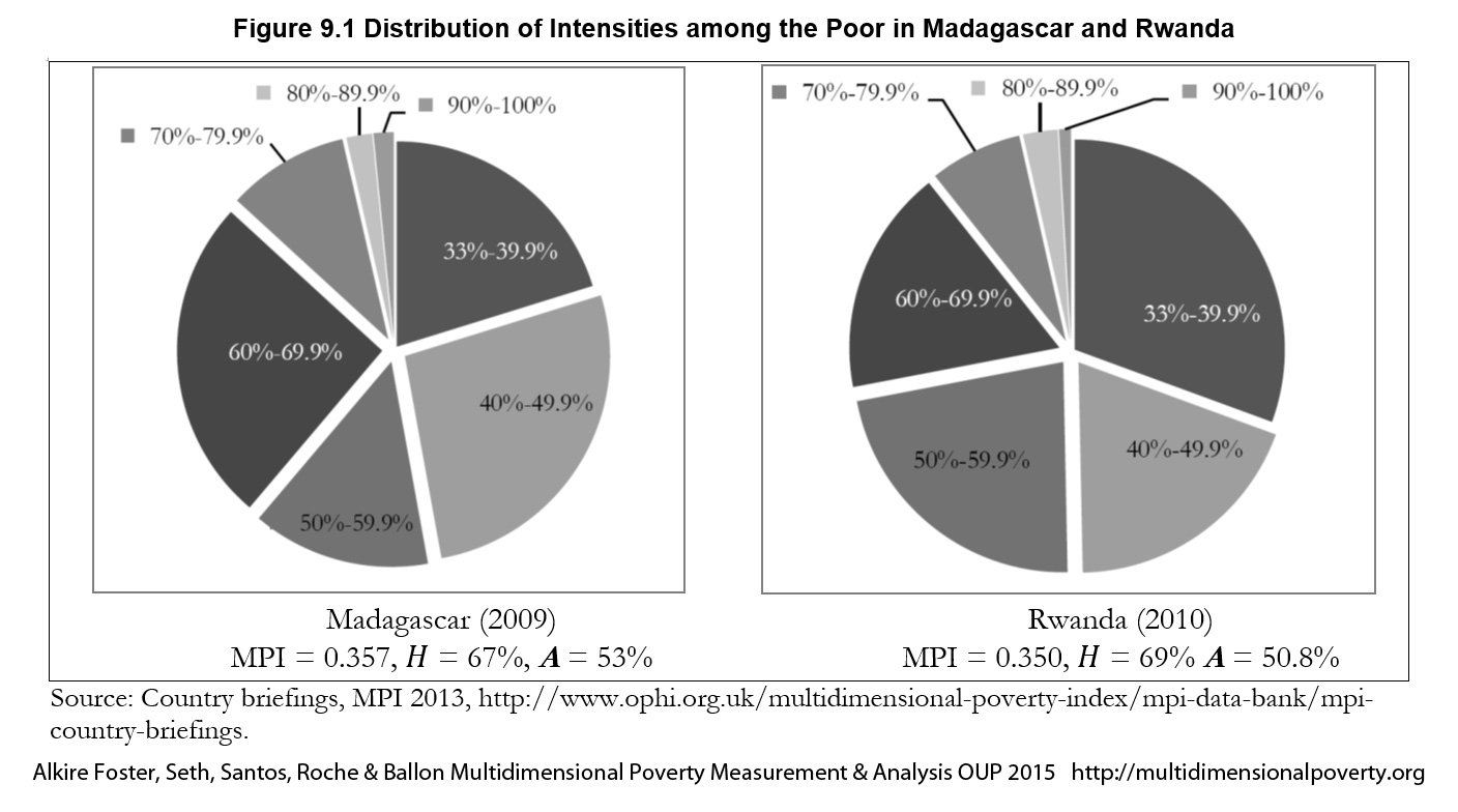
poor persons according to the value of their deprivation score ![]() and dividing them into groups. If the poverty cutoff is 30%, the analysis might then report the percentage of poor people whose deprivation scores fall in the band of 30–39.9% of deprivations, 40–49.9%, and so on to 100%. The percentage of people who experience different intensity gradients of poverty across regions and time can be compared to see how inequality among the poor is evolving.[7] Figure 9.1 presents an example of two countries—Madagascar and Rwanda—which have similar multidimensional headcount ratios (
and dividing them into groups. If the poverty cutoff is 30%, the analysis might then report the percentage of poor people whose deprivation scores fall in the band of 30–39.9% of deprivations, 40–49.9%, and so on to 100%. The percentage of people who experience different intensity gradients of poverty across regions and time can be compared to see how inequality among the poor is evolving.[7] Figure 9.1 presents an example of two countries—Madagascar and Rwanda—which have similar multidimensional headcount ratios (![]() ) and MPIs. However, the distributions of intensities across the poor are quite different. Also, data permitting, these intensity groups can be decomposed by population subgroups such as region or ethnicity. The comparisons can be enriched by applying a dimensional breakdown to examine the dimensional composition of poverty experienced by those having different ranges of deprivation scores.
) and MPIs. However, the distributions of intensities across the poor are quite different. Also, data permitting, these intensity groups can be decomposed by population subgroups such as region or ethnicity. The comparisons can be enriched by applying a dimensional breakdown to examine the dimensional composition of poverty experienced by those having different ranges of deprivation scores.
Figure 9.1 Distribution of Intensities among the Poor in Madagascar and Rwanda
9.1.3 Using a Separate Inequality Measure
Another tool is to supplement ![]() with a measure of inequality among the poor. Using the distribution of (censored) deprivation scores across the poor or some transformation of these, it is actually elementary to create an inequality measure, much in the same way that traditional inequality measures such as Atkinson, Theil, or Gini are constructed. Such measures will offer a window onto one type of multidimensional inequality—one that is oriented to the breadth of deprivations people experience. This approach is quite different from other constructions of multidimensional inequality, but it is useful, particularly when data are ordinal. Building on Chakravarty (2001), Seth and Alkire (2014a,b) propose such an inequality measure that is founded on certain properties. Note that these are properties of inequality measures, and are defined differently from those presented in Chapter 2 (despite similar names), but introduced intuitively below. Let us briefly discuss these properties before introducing the measure.
with a measure of inequality among the poor. Using the distribution of (censored) deprivation scores across the poor or some transformation of these, it is actually elementary to create an inequality measure, much in the same way that traditional inequality measures such as Atkinson, Theil, or Gini are constructed. Such measures will offer a window onto one type of multidimensional inequality—one that is oriented to the breadth of deprivations people experience. This approach is quite different from other constructions of multidimensional inequality, but it is useful, particularly when data are ordinal. Building on Chakravarty (2001), Seth and Alkire (2014a,b) propose such an inequality measure that is founded on certain properties. Note that these are properties of inequality measures, and are defined differently from those presented in Chapter 2 (despite similar names), but introduced intuitively below. Let us briefly discuss these properties before introducing the measure.
9.1.3.1 Properties
The first property, translation invariance, requires inequality not to change if the deprivation score of every poor person increases by the same amount. Implicitly, we assume that the measure reflects absolute inequality. Seth and Alkire (2014) argue that measures reflecting absolute inequality are more appropriate when each deprivation is judged to be of intrinsic importance. In addition, the use of the absolute inequality measure ensures that inequality remains the same whether poverty is measured by counting the number of deprivations or by counting the number of attainments. The use of the relative inequality measure is more common in the case of income inequality, where it is often assumed that as long as people’s relative incomes remain unchanged, inequality should not change. However, it is difficult to argue that inequality between two poor persons who are deprived in one and two dimensions respectively is the same as the inequality between two poor persons who are deprived in five and ten dimensions, respectively, if these deprivations referred to, for example, serious human rights violations. Any relative inequality measure, such as the Generalized Entropy measures (which include the Squared Coefficient of Variation associated with the FGT2 index) or Gini Coefficient, would evaluate these two situations as having identical inequality across the poor. Moreover, a relative inequality measure may provide counterintuitive conclusion while assessing inequality within a counting approach framework. In fact, no non-constant inequality measure exists that is simultaneously invariant to absolute as well as relative changes in a distribution.
The second property requires that the inequality measure should be additively decomposable so that overall inequality in any society can be broken down into within-group and between-group components. This can be quite useful for policy (Stewart 2010). We have shown in Chapter 5 that the additive structure of the indices in the AF class allows the overall poverty figure to be decomposed across various population subgroups. A country or a region with same level of overall poverty may have very different poverty levels across different subgroups, or a country may have the same level of poverty across two time periods, but the distribution of poverty across different subgroups may change over time. Furthermore, within each population subgroup, there may be different distributions of deprivation scores across poor persons living within that subgroup, thus reflecting various levels of within-group inequality.
The third property, within-group mean independence, requires that overall within-group inequality should be expressed as a weighted average of the subgroup inequalities, where the weight attached to a subgroup is equal to the population share of that subgroup. This assumption makes the interpretation and analysis of the inequality measure more intuitive.
Four additional properties are commonly satisfied when constructing any inequality measure. The anonymity property requires that a permutation of deprivation scores should not alter inequality. According to the replication invariance property, a mere replication of population leaves the inequality measure unaltered. The normalization property requires that the inequality measure should be equal to zero when the deprivation scores are equal for all. The transfer property requires that a progressive dimensional rearrangement among the poor should decrease inequality.
9.1.3.2 A Decomposable Measure
The proposed inequality measure, which is the only one to satisfy those properties, takes the general form
|
|
(9.1) |
where ![]() is a vector with
is a vector with ![]() elements. Relevant applications using our familiar notation will be provided in equations (9.6) and (9.7) below, but we first present the general form and notation. As we will show, in relevant applications an element
elements. Relevant applications using our familiar notation will be provided in equations (9.6) and (9.7) below, but we first present the general form and notation. As we will show, in relevant applications an element ![]() may be the deprivation score of a person
may be the deprivation score of a person ![]() or
or ![]() or the average poverty level of a region. The size of the vector
or the average poverty level of a region. The size of the vector ![]() for an entire population would be
for an entire population would be ![]() and for the poor it would be
and for the poor it would be ![]() The functional form in equation (9.1) is a positive multiple (
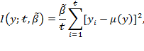
The functional form in equation (9.1) is a positive multiple (![]() ) of the variance. The measure reflects the average squared difference between person
) of the variance. The measure reflects the average squared difference between person ![]() ’s deprivation score and the mean of the deprivation scores in
’s deprivation score and the mean of the deprivation scores in ![]() . The value of parameter
. The value of parameter ![]() can be chosen in such a way that it normalizes the inequality measure to lie between 0 and 1.
can be chosen in such a way that it normalizes the inequality measure to lie between 0 and 1.
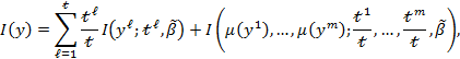
The overall inequality in ![]() may be decomposed into two components: total within-group inequality and between-group inequality. Following the notation in Chapter 2, suppose there are population subgroups. The deprivation score vector of subgroup
may be decomposed into two components: total within-group inequality and between-group inequality. Following the notation in Chapter 2, suppose there are population subgroups. The deprivation score vector of subgroup ![]() is denoted by
is denoted by ![]()
![]() with
with ![]() elements. The decomposition expression is given as follows:
elements. The decomposition expression is given as follows:
|
Total within-group Total between-group |
where ![]() is the population share of subgroup
is the population share of subgroup ![]() in the overall population and
in the overall population and ![]() is the mean of all elements in
is the mean of all elements in ![]() for all
for all ![]() .
.
The between-group inequality component ![]() in (9.2) can be computed as
in (9.2) can be computed as
|
|
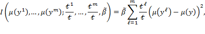
where ![]() is the mean of all elements in
is the mean of all elements in ![]() .
.
The within-group inequality component of subgroup ![]() can be computed using (9.1) as
can be computed using (9.1) as
|
|
(9.4) |
and thus the total within-group inequality component in (9.2) can be computed as
|
|
9.1.3.3 Two Important Applications
There are different relevant applications of this inequality framework to multidimensional poverty analyses based on ![]() . The first central case is to assess inequality among the poor. To do so we suppose that the deprivation scores are ordered in a descending order and the first
. The first central case is to assess inequality among the poor. To do so we suppose that the deprivation scores are ordered in a descending order and the first ![]() persons are identified as poor. The elements are taken from the censored deprivation score vector,
persons are identified as poor. The elements are taken from the censored deprivation score vector, ![]() We choose vector
We choose vector ![]() such that it contains only the deprivation scores of the poor (
such that it contains only the deprivation scores of the poor (![]() ). The average of all elements in
). The average of all elements in ![]() then is the intensity of poverty which for
then is the intensity of poverty which for ![]() persons is
persons is ![]() . We can then denote the inequality measure that reflects inequality in multiple deprivations only among the poor by
. We can then denote the inequality measure that reflects inequality in multiple deprivations only among the poor by ![]() , which can be expressed as
, which can be expressed as
|
|

The ![]() measure effectively summarizes the information underlying Figure 9.1. It goes well beyond that figure because each individual deprivation score is used, which effectively creates a much finer gradation of intensity than that figure portrays. Furthermore, it can be decomposed by subgroup, to permit comparisons of within-subgroup inequalities among the poor. It can also be used over time to show how inequality among the poor changed.
measure effectively summarizes the information underlying Figure 9.1. It goes well beyond that figure because each individual deprivation score is used, which effectively creates a much finer gradation of intensity than that figure portrays. Furthermore, it can be decomposed by subgroup, to permit comparisons of within-subgroup inequalities among the poor. It can also be used over time to show how inequality among the poor changed.
Our second central case considers inequalities in poverty levels across population subgroups. It is motivated by studies of horizontal inequalities that find group-based inequalities to predict tension and in some cases conflict (Stewart 2010). Essentially, the measure reflects population-weighted disparities in poverty levels across population subgroups.
Suppose the censored deprivation score vector of subgroup ![]() is denoted by
is denoted by ![]() with
with ![]() elements. If instead of only considering the deprivation scores of the poor, we now sum across the whole population so (
elements. If instead of only considering the deprivation scores of the poor, we now sum across the whole population so (![]() ), then we realize that
), then we realize that ![]() or the average of all elements in
or the average of all elements in ![]() is actually the
is actually the ![]() of subgroup
of subgroup ![]() , which for simplicity we denote by
, which for simplicity we denote by ![]() . The between-group component of
. The between-group component of ![]() shows the disparity in the national Adjusted Headcount Ratio
shows the disparity in the national Adjusted Headcount Ratio ![]() across subgroups and is written using (9.3) as
across subgroups and is written using (9.3) as
|
|
Thus, equation (9.7) captures the disparity in ![]() s across
s across ![]() population subgroups, which can be used to detect patterns in horizontal disparities over time. Naturally, the number and population share of the subgroups must be considered in such comparisons.
population subgroups, which can be used to detect patterns in horizontal disparities over time. Naturally, the number and population share of the subgroups must be considered in such comparisons.
While studying disparity in MPIs across sub-national regions, Alkire, Roche, and Seth (2011) found that the national MPIs masked a large amount of sub-national disparity within countries, and Alkire and Seth (2013) and Alkire, Roche, and Vaz (2014) found considerable disparity in poverty trends across subnational groups. In some countries, the overall situation of the poor improved, but not all subgroups shared the equal fruit of success in poverty reduction and indeed poverty levels may have stagnated or risen in some groups. Therefore, it is also important to look at inequality or disparity in poverty across population subgroups. This separate inequality measure, elaborated in Seth and Alkire (2014), provides such framework.
9.1.3.4 An Illustration
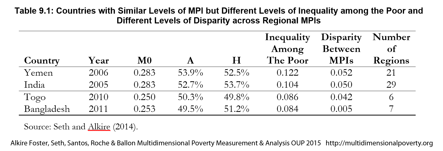
Table 9.1 presents two pair-wise comparisons. For the inequality measure, we choose ![]() 4 because the deprivation scores are bounded between 0 and 1; hence the maximum possible variance is 0.25.
4 because the deprivation scores are bounded between 0 and 1; hence the maximum possible variance is 0.25. ![]() 4 ensures that the inequality measure lies between 0 and 1. The first pair of countries, India and Yemen, have exactly the same levels of MPI. The multidimensional headcount ratios and the intensities of poverty are also similar. However, the inequality among the poor (computed using equation (9.1)) is much higher in Yemen than in India. We also measure disparity across sub-national regions. Yemen has twenty-one sub-national regions whereas, India has twenty-nine sub-national regions. We find that, like the national MPIs, the disparities across subnational MPIs—computed using equation 9.7)—are similar. This means that the inequality in Yemen is not primarily due to regional disparities in poverty levels, but may be affected by non-geographic divides such as cultural or rural–urban.
4 ensures that the inequality measure lies between 0 and 1. The first pair of countries, India and Yemen, have exactly the same levels of MPI. The multidimensional headcount ratios and the intensities of poverty are also similar. However, the inequality among the poor (computed using equation (9.1)) is much higher in Yemen than in India. We also measure disparity across sub-national regions. Yemen has twenty-one sub-national regions whereas, India has twenty-nine sub-national regions. We find that, like the national MPIs, the disparities across subnational MPIs—computed using equation 9.7)—are similar. This means that the inequality in Yemen is not primarily due to regional disparities in poverty levels, but may be affected by non-geographic divides such as cultural or rural–urban.
A contrasting finding for regional disparity is obtained across Togo and Bangladesh. As before, the MPIs, headcount ratios, and intensities are quite similar across two countries—but with two differences. The inequality among the poor is very similar, but the regional disparities are stark. Even though both countries have similar number of sub-national regions, the level of sub-national disparity is much higher in Togo than that in Bangladesh.
Table 9.1: Countries with Similar Levels of MPI but Different Levels of Inequality among the Poor and Different Levels of Disparity across Regional MPIs
9.2 Descriptive Analysis of Changes over Time
A strong motivation for computing multidimensional poverty is to track and analyse changes over time. Most data available to study changes over time are repeated cross-sectional data, which compare the characteristics of representative samples drawn at different periods with sampling errors, but do not track specific individuals across time. This section describes how to compare ![]() and its associated partial indices over time with repeated cross-sectional data. It offers a standard methodology of computing such changes, and an array of small examples. This section does not treat the data issues underlying poverty comparisons, and readers are expected to know standard techniques that are required for such rigorous empirical comparisons. For example, the definition of indicators, cutoffs, weights, etc. must be strictly harmonized for meaningful comparisons across time, which always requires close verification of survey questions and response structures, and may require amending or dropping indicators. The sample designs of the surveys must be such that they can be meaningfully compared, and basic issues like the representativeness and structure of the data must be thoroughly understood and respected. We presume this background in what follows. This section focuses on changes across two time periods; naturally the comparisons can be easily extended across more than two time periods.
and its associated partial indices over time with repeated cross-sectional data. It offers a standard methodology of computing such changes, and an array of small examples. This section does not treat the data issues underlying poverty comparisons, and readers are expected to know standard techniques that are required for such rigorous empirical comparisons. For example, the definition of indicators, cutoffs, weights, etc. must be strictly harmonized for meaningful comparisons across time, which always requires close verification of survey questions and response structures, and may require amending or dropping indicators. The sample designs of the surveys must be such that they can be meaningfully compared, and basic issues like the representativeness and structure of the data must be thoroughly understood and respected. We presume this background in what follows. This section focuses on changes across two time periods; naturally the comparisons can be easily extended across more than two time periods.
9.2.1 Changes in M0, H and A across Two Time Periods
The basic component of poverty comparisons is the absolute pace of change across periods.[10] The absolute rate of change is the difference in levels between two periods. Changes (increases or decreases) in poverty across two time periods can also be reported as a relative rate. The relative rate of change is the difference in levels across two periods as a percentage of the initial period.
For example, if the ![]() has gone down from 0.5 to 0.4 between two consecutive years, then the absolute rate of change is (0.5 – 0.4) = 0.1. It tells us how much level of poverty (
has gone down from 0.5 to 0.4 between two consecutive years, then the absolute rate of change is (0.5 – 0.4) = 0.1. It tells us how much level of poverty (![]() ) has changed: 10% of the total possible set of deprivations that poor people in that society could have experienced has been eradicated; 40% remains. The relative rate of change is (0.5 – 0.4)/0.5 = 20%, which tells us that
) has changed: 10% of the total possible set of deprivations that poor people in that society could have experienced has been eradicated; 40% remains. The relative rate of change is (0.5 – 0.4)/0.5 = 20%, which tells us that ![]() has gone down by 20% with respect to the initial level. While absolute changes are in some sense prior, because they are easy to understand and compare, both absolute and relative rates may be important to report and analyse. The value-added of the relative changes is evident in relatively low-poverty regions. A region or country with a high initial level of poverty may be able to reduce poverty in absolute terms much more than one having a low initial level of poverty. It is however possible that although a region or country with low initial poverty levels did not show a large absolute reduction, the reduction was large relative to its initial level and thus it should not be discounted for its slower absolute reduction.[11] The analysis of both absolute and relative changes gives a clear sense of overall progress.
has gone down by 20% with respect to the initial level. While absolute changes are in some sense prior, because they are easy to understand and compare, both absolute and relative rates may be important to report and analyse. The value-added of the relative changes is evident in relatively low-poverty regions. A region or country with a high initial level of poverty may be able to reduce poverty in absolute terms much more than one having a low initial level of poverty. It is however possible that although a region or country with low initial poverty levels did not show a large absolute reduction, the reduction was large relative to its initial level and thus it should not be discounted for its slower absolute reduction.[11] The analysis of both absolute and relative changes gives a clear sense of overall progress.
In expressing changes across two periods, we denote the initial period by ![]() and the final period by
and the final period by ![]() . This section mostly presents the expressions for
. This section mostly presents the expressions for ![]() , but they are equally applicable to its partial indices: incidence (
, but they are equally applicable to its partial indices: incidence (![]() ), intensity (
), intensity (![]() ), censored headcount ratios (
), censored headcount ratios (![]() ), and uncensored headcount ratios (
), and uncensored headcount ratios (![]() ). The achievement matrices for period
). The achievement matrices for period ![]() and
and ![]() are denoted by
are denoted by ![]() and
and ![]() , respectively. As presented in Chapter 5,
, respectively. As presented in Chapter 5, ![]() and its partial indices depend on a set of parameters: deprivation cutoff vector
and its partial indices depend on a set of parameters: deprivation cutoff vector ![]() , weight vector
, weight vector ![]() and poverty cutoff
and poverty cutoff ![]() . For simplicity of notation though, we present
. For simplicity of notation though, we present ![]() and its partial indices only as a function of the achievement matrix. For strict intertemporal comparability, it is important that the same set of parameters be used across two periods.
and its partial indices only as a function of the achievement matrix. For strict intertemporal comparability, it is important that the same set of parameters be used across two periods.
The absolute rate of change (![]() ) is simply the difference in Adjusted Headcount Ratios between two periods and is computed as
) is simply the difference in Adjusted Headcount Ratios between two periods and is computed as
|
|
Similarly, for ![]() and
and ![]() :
:
|
|
|
|
The relative rate of change (![]() ) is the difference in Adjusted Headcount Ratios as a percentage of the initial poverty level and is computed for
) is the difference in Adjusted Headcount Ratios as a percentage of the initial poverty level and is computed for![]() and
and ![]() (only
(only ![]() shown) as
shown) as
|
|
If one is interested in comparing changes over time for the same reference period, the expressions (5.7) and (9.11) are appropriate. However, in cross-country exercises, one may often be interested in comparing the rates of poverty reduction across countries that have different periods of references. For example the reference period of one country may be five years; whereas the reference period for another country is three years. It is evident in Table 9.2 that the reference period of Nepal is five years (2006–2011); whereas that of Peru is only three years (2005-–2008). In such cases, it is essential to annualize the change in order to preserve strict comparison.
The annualized absolute rate of change (![]() ) is the difference in Adjusted Headcount Ratios between two periods divided by the difference in the two time periods (
) is the difference in Adjusted Headcount Ratios between two periods divided by the difference in the two time periods (![]() ) and is computed for
) and is computed for ![]() as
as
|
|
The annualized relative rate of change (![]() ) is the compound rate of reduction in
) is the compound rate of reduction in ![]() per year between the initial and the final periods, and is computed for
per year between the initial and the final periods, and is computed for ![]() as
as
|
|
As formula (9.8) has been used to compute the changes in ![]() and
and ![]() using formulae (9.9) and (9.10), formulae (9.11) to (9.13) can be used to compute and report annualized changes in the other partial indices, namely
using formulae (9.9) and (9.10), formulae (9.11) to (9.13) can be used to compute and report annualized changes in the other partial indices, namely ![]() ,
,![]() ,
, ![]() or
or ![]()
9.2.2 An Example: Analyzing Changes in Global MPI for Four Countries
Table 9.2 presents both the annualized absolute and annualized relative rates of change in Global MPI, as outlined in Chapter 5, and its two partial indices—![]() and
and ![]() —for four countries: Nepal, Peru, Rwanda, and Senegal, drawing from Alkire, Roche and Vaz (2014). Taking the survey design into account, we also present the standard errors (in parentheses) and the levels of statistical significance of the rates of reduction, as described in the Appendix of Chapter 8. The figures in the first four columns present the values and standard errors for
—for four countries: Nepal, Peru, Rwanda, and Senegal, drawing from Alkire, Roche and Vaz (2014). Taking the survey design into account, we also present the standard errors (in parentheses) and the levels of statistical significance of the rates of reduction, as described in the Appendix of Chapter 8. The figures in the first four columns present the values and standard errors for ![]() ,
, ![]() and
and ![]() in both time periods. The results show that Peru had the lowest MPI with 0.085 in the initial year, while Rwanda had the highest with 0.460.
in both time periods. The results show that Peru had the lowest MPI with 0.085 in the initial year, while Rwanda had the highest with 0.460.
Under the heading ‘annualized change’, Table 9.2 provides the annualized absolute and annualized relative reduction for ![]() ,
, ![]() and
and ![]() , which are computed using equations (9.12) and (9.13). It shows, for example, that Nepal with a much lower initial poverty level than Rwanda, has experienced a greater absolute annualized poverty reduction of ‒0.027. In relative terms Nepal outperformed Rwanda. Peru had a low initial poverty level, and reduced it in absolute terms by only ‒0.006 per year, which means that the share of all possible deprivations among poor people that were removed was only less than one-fourth that of Nepal or Rwanda. But relative to its initial level of poverty, its progress was second only to Nepal. It is thus important to report both absolute and relative changes and to understand their interpretation. The same results for
, which are computed using equations (9.12) and (9.13). It shows, for example, that Nepal with a much lower initial poverty level than Rwanda, has experienced a greater absolute annualized poverty reduction of ‒0.027. In relative terms Nepal outperformed Rwanda. Peru had a low initial poverty level, and reduced it in absolute terms by only ‒0.006 per year, which means that the share of all possible deprivations among poor people that were removed was only less than one-fourth that of Nepal or Rwanda. But relative to its initial level of poverty, its progress was second only to Nepal. It is thus important to report both absolute and relative changes and to understand their interpretation. The same results for ![]() and
and ![]() are provided in the Panel II and III of the table. We see that Nepal reduced the percentage of people who were poor by 4.1 percentage points per year—for example, if the first year 64.7% of people were poor, the next year it would be 60.6%. Peru cut the poverty incidence by 1.3 percentage points per year. Relative to their starting levels, they had similar relative rates of reduction of the headcount ratio. Note that when estimates are reported in percentages, the absolute changes are reported in ‘percentage points’ and not in ‘percentages’. Thus, Nepal’s reduction in
are provided in the Panel II and III of the table. We see that Nepal reduced the percentage of people who were poor by 4.1 percentage points per year—for example, if the first year 64.7% of people were poor, the next year it would be 60.6%. Peru cut the poverty incidence by 1.3 percentage points per year. Relative to their starting levels, they had similar relative rates of reduction of the headcount ratio. Note that when estimates are reported in percentages, the absolute changes are reported in ‘percentage points’ and not in ‘percentages’. Thus, Nepal’s reduction in ![]() from 64.7% to 44.2% is equivalent to an annualized absolute reduction of 4.1 percentage points and an annualized relative reduction of 6.3%.
from 64.7% to 44.2% is equivalent to an annualized absolute reduction of 4.1 percentage points and an annualized relative reduction of 6.3%.
Table 9.2: Reduction in Multidimensional Poverty Index, Headcount Ratio and Intensity of Poverty in Nepal, Peru, Rwanda and Senegal
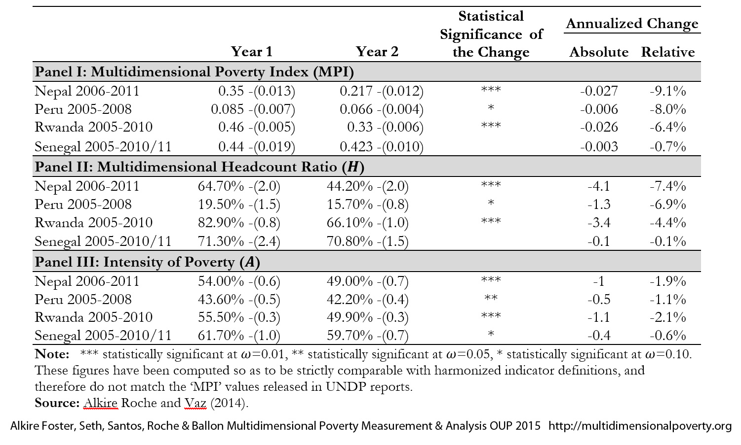
The third column provides the results for the hypothesis tests which assess if the reduction between both years is statistically significant.[12] The reductions in ![]() in Nepal and Rwanda are significant at
in Nepal and Rwanda are significant at ![]() =0.01, but the same in Peru is only significant at
=0.01, but the same in Peru is only significant at ![]() =0.10. Interestingly, the reduction in intensity of poverty in Peru is significant at
=0.10. Interestingly, the reduction in intensity of poverty in Peru is significant at ![]() =0.05. The case of Senegal is different in that the small reduction in
=0.05. The case of Senegal is different in that the small reduction in ![]() is not even significantly different at
is not even significantly different at ![]() =0.10, preventing the null hypothesis that poverty level in both years remained unchanged from being rejected.
=0.10, preventing the null hypothesis that poverty level in both years remained unchanged from being rejected.
9.2.3 Population Growth and Change in the Number of Multidimensionally Poor
Besides comparing the rate of reduction in ![]() ,
, ![]() and
and ![]() as in Table 9.2, one should also examine whether the number of poor people is decreasing over time. It may be possible that the population growth is large enough to offset the rate of poverty reduction. Table 9.3 uses the same four countries as Table 9.2 but adds demographic information. Nepal had an annual population growth of 1.2% between 2006 and 2011, moving from 25.6 to 27.2 million people, and reduced the headcount ratio from 64.7% to 44.2%. This means that Nepal reduced the absolute number of poor by 4.6 million between 2006 and 2011.
as in Table 9.2, one should also examine whether the number of poor people is decreasing over time. It may be possible that the population growth is large enough to offset the rate of poverty reduction. Table 9.3 uses the same four countries as Table 9.2 but adds demographic information. Nepal had an annual population growth of 1.2% between 2006 and 2011, moving from 25.6 to 27.2 million people, and reduced the headcount ratio from 64.7% to 44.2%. This means that Nepal reduced the absolute number of poor by 4.6 million between 2006 and 2011.
Table 9.3 Changes in the Number of Poor Accounting for Population Growth
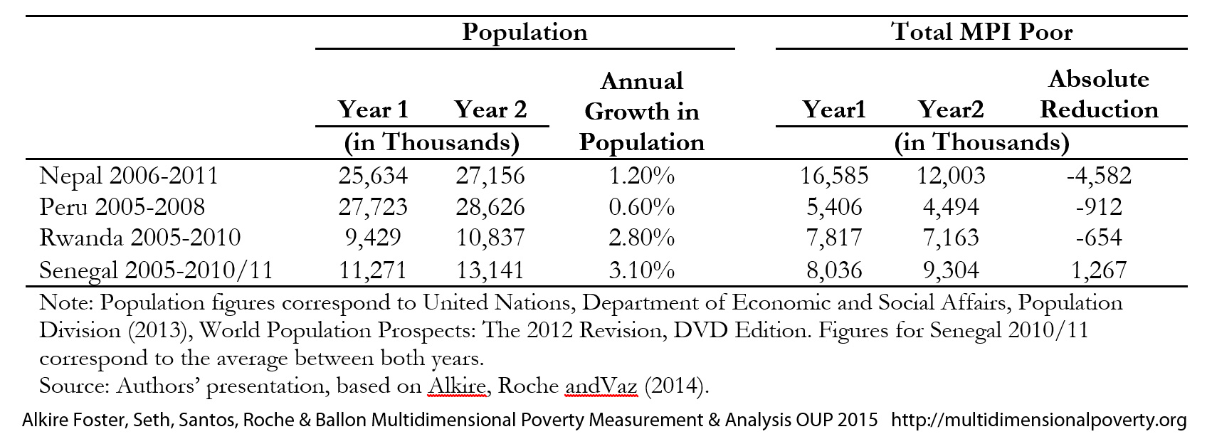 In order to reduce the absolute number of poor people, the rate of reduction in the headcount ratio needs to be faster than the population growth. The largest reduction in the number of multidimensionally poor has taken place in Nepal. A moderate reduction in the number of poor has taken place in Peru and Rwanda. In contrast, there has been an increase in the total number of multidimensional poor in Senegal, from 8 million to over 9 million between 2005 and 2011.
9.2.4 Dimensional Changes (Uncensored and Censored Headcount Ratios)
The reductions in ![]() ,
, ![]() , or
, or ![]() can be broken down to reveal which dimensions have been responsible for the change in poverty. This can be seen by looking at changes in the uncensored headcount ratios (
can be broken down to reveal which dimensions have been responsible for the change in poverty. This can be seen by looking at changes in the uncensored headcount ratios (![]() ) and censored headcount ratios (
) and censored headcount ratios (![]() ) described in section 5.5.3. We present the uncensored and censored headcount ratios of MPI indicators for Nepal in Table 9.4 for years 2006 and 2011 and analyse their changes over time. For definitions of indicators and their deprivation cutoffs, see section 5.6. Panel I gives levels and changes in uncensored headcount ratios, i.e. the percentage of people that are deprived in each indicator irrespective of deprivations in other indicators. Panel II provides levels and changes in the censored headcount ratios, i.e. the percentage of people that are multidimensionally poor and simultaneously deprived in each indicator. By definition, the uncensored headcount ratio of an indicator is equal to or higher than the censored headcount of that indicator. The standard errors are reported in the parenthesis.
) described in section 5.5.3. We present the uncensored and censored headcount ratios of MPI indicators for Nepal in Table 9.4 for years 2006 and 2011 and analyse their changes over time. For definitions of indicators and their deprivation cutoffs, see section 5.6. Panel I gives levels and changes in uncensored headcount ratios, i.e. the percentage of people that are deprived in each indicator irrespective of deprivations in other indicators. Panel II provides levels and changes in the censored headcount ratios, i.e. the percentage of people that are multidimensionally poor and simultaneously deprived in each indicator. By definition, the uncensored headcount ratio of an indicator is equal to or higher than the censored headcount of that indicator. The standard errors are reported in the parenthesis.
Table 9.4: Uncensored and Censored Headcount Ratios of the Global MPI, Nepal 2006–2011
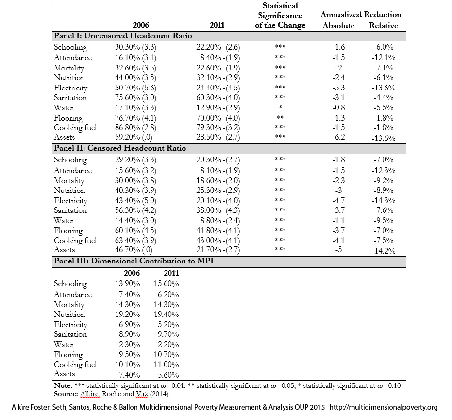 As we can see in the table, Nepal made statistically significant reductions in all indicators in terms of both uncensored and censored headcount ratios. The larger reductions in censored headcount are observed in electricity, assets, cooking fuel, flooring, and sanitation; all censored headcount ratios have decreased by more than 3 percentage points. Nutrition, mortality, schooling and attendance follow with annual reductions of 3, 2.3, 1.8, and 1.5 percentage points, respectively.
The changes in censored headcount ratios depict changes in deprivations among the poor. Recall that the overall ![]() is the weighted sum of censored headcount ratios of the indicators as presented in equation (5.13) and the contribution of each indicator to the
is the weighted sum of censored headcount ratios of the indicators as presented in equation (5.13) and the contribution of each indicator to the ![]() can be computed by equation (5.14). Because of this relationship, the absolute rate of reduction in
can be computed by equation (5.14). Because of this relationship, the absolute rate of reduction in ![]() in equation (9.8) and the annualized absolute rate of reduction in
in equation (9.8) and the annualized absolute rate of reduction in ![]() in equation (9.12) can be expressed as weighted averages of absolute rate of reductions in censored headcount ratios and annualized absolute rate of reductions in censored headcount ratios, respectively. When different indicators are assigned different weights, the effects of their changes on the change in
in equation (9.12) can be expressed as weighted averages of absolute rate of reductions in censored headcount ratios and annualized absolute rate of reductions in censored headcount ratios, respectively. When different indicators are assigned different weights, the effects of their changes on the change in ![]() reflect these weights.[13] For example, in the MPI, the nutrition indicator is assigned a three times more weight than electricity. This implies that a one percentage point reduction in nutrition ceteris paribus would lead to an absolute reduction in
reflect these weights.[13] For example, in the MPI, the nutrition indicator is assigned a three times more weight than electricity. This implies that a one percentage point reduction in nutrition ceteris paribus would lead to an absolute reduction in ![]() that is three times larger than a one percentage point reduction in the electricity indicator.
that is three times larger than a one percentage point reduction in the electricity indicator.
Recall that it is straightforward to compute the contribution of each indicator to ![]() using its weighted censored headcount ratio as given in equation (5.14). Note that interpreting the real on-the-ground contribution of each indicator to the change in
using its weighted censored headcount ratio as given in equation (5.14). Note that interpreting the real on-the-ground contribution of each indicator to the change in ![]() is not so mechanical. Why? A reduction in the censored headcount ratio of an indicator is not independent of the changes in other indicators. It is possible that the reduction in the censored headcount ratio of a certain indicator
is not so mechanical. Why? A reduction in the censored headcount ratio of an indicator is not independent of the changes in other indicators. It is possible that the reduction in the censored headcount ratio of a certain indicator ![]() occurred because a poor person became non-deprived in indicator
occurred because a poor person became non-deprived in indicator ![]() But it is also possible that the reduction occurred because a person who had been deprived in
But it is also possible that the reduction occurred because a person who had been deprived in ![]() became non-poor due to reductions in other indicators, even though they remain deprived in
became non-poor due to reductions in other indicators, even though they remain deprived in ![]() . In the second period, their deprivation in
. In the second period, their deprivation in ![]() is now censored because they are non-poor (their deprivation score does not exceed
is now censored because they are non-poor (their deprivation score does not exceed ![]() ). The comparison between the uncensored and censored headcount distinguishes these situations. For example, we can see from Panel I of Table 9.4 that the reductions in the uncensored headcount ratios of flooring and cooking fuel are lower than the annualized reductions of the censored headcount ratios of the these two indicators. Thus some non-poor people are deprived in these indicators. In intertemporal analysis it is useful to compare the corresponding censored and uncensored headcount ratios to analyse the relation between the dimensional changes among the poor and the society-wide changes in deprivations. Of course in repeated cross-sectional data, this comparison will also be affected by migration and demographic shifts as well as changes in the deprivation profiles of the non-poor.
). The comparison between the uncensored and censored headcount distinguishes these situations. For example, we can see from Panel I of Table 9.4 that the reductions in the uncensored headcount ratios of flooring and cooking fuel are lower than the annualized reductions of the censored headcount ratios of the these two indicators. Thus some non-poor people are deprived in these indicators. In intertemporal analysis it is useful to compare the corresponding censored and uncensored headcount ratios to analyse the relation between the dimensional changes among the poor and the society-wide changes in deprivations. Of course in repeated cross-sectional data, this comparison will also be affected by migration and demographic shifts as well as changes in the deprivation profiles of the non-poor.
Panel III of Table 9.5 presents the contribution of the indicators to the ![]() for Nepal in 2006 and in 2011. The contributions of assets, electricity, and attendance have gone down; whereas the contributions of flooring, cooking fuel, sanitation, and schooling have gone up. The contributions of water, nutrition and mortality have not shown large changes. Dimensional analyses is vital and motivating because any real reduction in a dimensional deprivation will certainly reduce
for Nepal in 2006 and in 2011. The contributions of assets, electricity, and attendance have gone down; whereas the contributions of flooring, cooking fuel, sanitation, and schooling have gone up. The contributions of water, nutrition and mortality have not shown large changes. Dimensional analyses is vital and motivating because any real reduction in a dimensional deprivation will certainly reduce ![]() . Real reductions are normally those which are visible both in raw and censored headcounts.[14]
. Real reductions are normally those which are visible both in raw and censored headcounts.[14]
9.2.5 Subgroup Decomposition of Change in Poverty
One important property that the adjusted-FGT measures satisfy is population subgroup decomposability, so that the overall ![]() can be expressed as:
can be expressed as: ![]() where
where![]() denotes the Adjusted Headcount Ratio and
denotes the Adjusted Headcount Ratio and ![]() the population share of subgroup
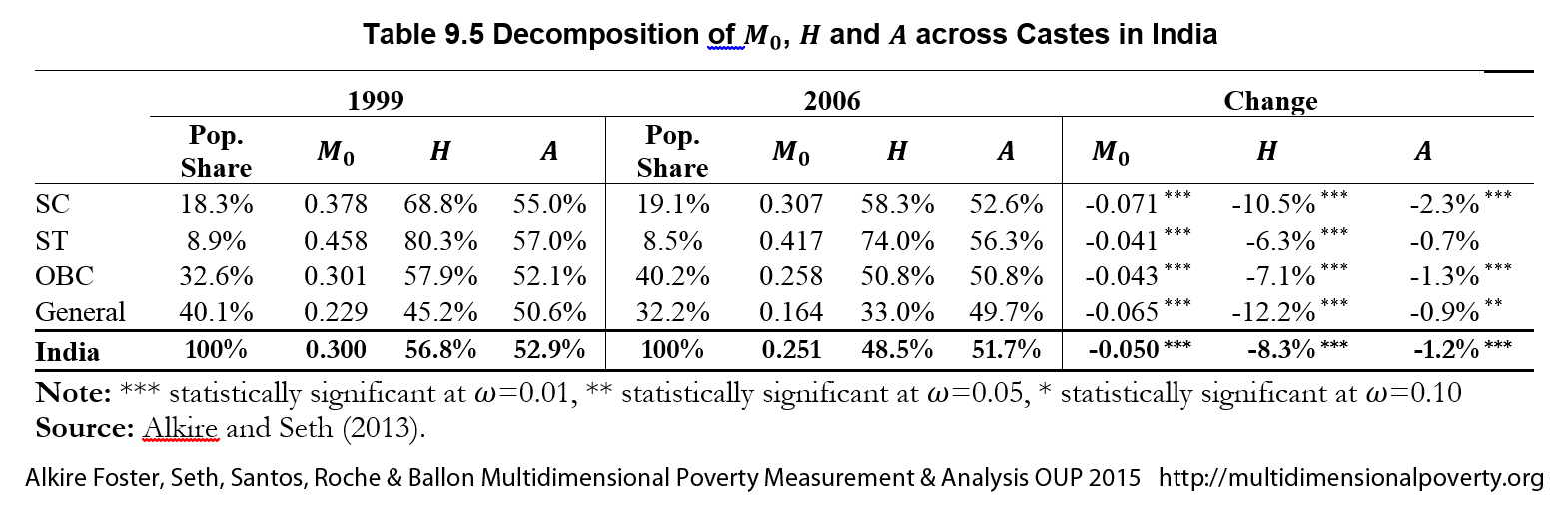
the population share of subgroup ![]() as in equation (5.14). It is extremely useful to analyse poverty changes by population subgroups, to see if the poorest subgroups reduced poverty faster than less poor subgroups, and to see the dimensional composition of reduction across subgroups (Alkire and Seth 2013b; Alkire and Roche 2013; Alkire, Roche and Vaz 2014). Population shares for each time period must be analysed alongside subgroup trends. For example, let us decompose the Indian population into four caste categories: Scheduled Castes (SC), Scheduled Tribes (ST), Other Backward Classes (OBC), and the General category. As Table 9.5 shows,
as in equation (5.14). It is extremely useful to analyse poverty changes by population subgroups, to see if the poorest subgroups reduced poverty faster than less poor subgroups, and to see the dimensional composition of reduction across subgroups (Alkire and Seth 2013b; Alkire and Roche 2013; Alkire, Roche and Vaz 2014). Population shares for each time period must be analysed alongside subgroup trends. For example, let us decompose the Indian population into four caste categories: Scheduled Castes (SC), Scheduled Tribes (ST), Other Backward Classes (OBC), and the General category. As Table 9.5 shows, ![]() as well as
as well as ![]() have gone down statistically significantly at the national level and across all four subgroups, which is good news. However, the reduction was slowest among STs who were the poorest as a group in 1999, and their intensity showed no significant decrease. Thus, the poorest subgroup registered slowest progress in terms of reducing poverty.
have gone down statistically significantly at the national level and across all four subgroups, which is good news. However, the reduction was slowest among STs who were the poorest as a group in 1999, and their intensity showed no significant decrease. Thus, the poorest subgroup registered slowest progress in terms of reducing poverty.
Table 9.5 Decomposition of ![]() ,
, ![]() and
and ![]() across Castes in India
across Castes in India
 To supplement the above analysis it is useful to explore the contribution of population subgroups to the overall reduction in poverty, which not only depends on the changes in subgroups’ poverty but also on changes in the population composition. This can be seen by presenting the overall change in
 ![]() between two periods (
between two periods (![]() ) as
) as
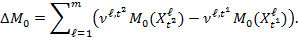
Note that the overall change depends both on the changes in subgroup ![]() ’s and the changes in population shares of the subgroups.
’s and the changes in population shares of the subgroups.
9.3 Changes Over Time by Dynamic Subgroups
The overall changes in ![]() and
and ![]() discussed thus far could have been generated in many ways. It might be desirable for policy purposes to monitor how poverty changed. In particular, one may wish to pinpoint the extent to which poverty reduction occurred due to people leaving poverty vs. a reduction of intensity among those who remained poor, and also to know the precise dimensional changes which drove each.
discussed thus far could have been generated in many ways. It might be desirable for policy purposes to monitor how poverty changed. In particular, one may wish to pinpoint the extent to which poverty reduction occurred due to people leaving poverty vs. a reduction of intensity among those who remained poor, and also to know the precise dimensional changes which drove each.
For example, a decrease in the headcount ratio by 10% could have been generated by an exit of 10% of the population who had been poor in the first period. Alternatively, it could have been generated by a 20% decrease in the population who had been poor, accompanied by an influx of 10% of the population who became newly poor. Furthermore, the people who exited poverty could have had high deprivation scores in the first period – that is, been among the poorest – or they could have been only barely poor. The deprivation scores of those entering and leaving poverty will affect the overall change in intensity ![]() as will changes among those who stay poor. In addition these entries into and exits from poverty could have been precipitated by diferent possible increases or decreases in the dimensional deprivations people experienced in the first period, which will then be reflected in the changes in uncensored and censored headcount ratios.
as will changes among those who stay poor. In addition these entries into and exits from poverty could have been precipitated by diferent possible increases or decreases in the dimensional deprivations people experienced in the first period, which will then be reflected in the changes in uncensored and censored headcount ratios.
This section introduces more precisely these dynamics of change. We first show what can be captured with panel data, then show empirical strategies to address this situation with repeated cross-sectional data. Finally we present two approaches related to Shapley decompositions which decompose changes precisely, but rely on some crucial assumptions so their empirical accuracy is questionable.
9.3.1 Exits, Entries, and the Ongoing Poor: A Two-Period Panel
Let us consider a fixed set of population of size ![]() across two periods,
across two periods, ![]() and
and ![]() . The achievement matrices of these periods are denoted by
. The achievement matrices of these periods are denoted by ![]() and
and ![]() . The population can be mutually exclusively and collectively exhaustively categorized into four groups that we refer to as dynamic subgroups as follows:
. The population can be mutually exclusively and collectively exhaustively categorized into four groups that we refer to as dynamic subgroups as follows:
|
Subgroup |
Contains |
|
Subgroup |
Contains |
|
Subgroup |
Contains |
|
Subgroup |
Contains |
We denote the achievement matrices of these four subgroups in period ![]() by
by ![]() ,
, ![]() ,
, ![]() and
and ![]() for all
for all ![]() ,
, ![]() . The proportion of multidimensionally poor populationin period
. The proportion of multidimensionally poor populationin period ![]() is
is ![]() and that in period
and that in period ![]() is
is ![]() . The change in the proportion of poor people between these two periods is
. The change in the proportion of poor people between these two periods is ![]() =
=![]() . In other words, the change in the overall multidimensional headcount ratio is the difference between the proportion of poor entering and the proportion of poor exiting poverty. Note that, by construction, no person is poor in
. In other words, the change in the overall multidimensional headcount ratio is the difference between the proportion of poor entering and the proportion of poor exiting poverty. Note that, by construction, no person is poor in ![]() ,
, ![]() ,
, ![]() , and
, and ![]() and thus
and thus ![]() . This also implies,
. This also implies, ![]() . On the other hand, all persons in
. On the other hand, all persons in ![]() ,
, ![]() ,
, ![]() , and
, and ![]() are poor and thus
are poor and thus ![]() . Therefore, the
. Therefore, the ![]() of each of these four subgroups is equal to its intensity of poverty.
of each of these four subgroups is equal to its intensity of poverty.
In a fixed population, the overall population and the population share of each dynamic group remains unchanged across two time periods.[15] The change in the overall ![]() can be decomposed using equation (9.14) as
can be decomposed using equation (9.14) as
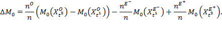
Thus, the right-hand side of equation (9.15) has three components. The first component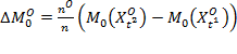 is due to the change in the intensity of those who remain poor in both periods—the ongoing poor—weighted by the size of this dynamic subgroup. The second component
 ![]() is due to the change in the intensity of those who exit poverty (weighted by the size of this subgroup) and the third component
is due to the change in the intensity of those who exit poverty (weighted by the size of this subgroup) and the third component 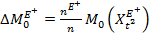 is due to the population-weighted change in the intensity of those who enter poverty. Together
 ![]() .
.
From this point there are many interesting possible avenues for analyses. Each group can be studied separately or in different combinations. For policy, it could be interesting to know who exited poverty, and their intensity in the previous period, to see if the poorest of the poor moved out of poverty. The intensity of those who entered poverty shows whether they dipped into the barely poor group, or catapulted into high-intensity poverty, perhaps due to some shock or crisis or (if the population is not fixed) migration. Intensity changes among the ongoing poor show whether their deprivations are declining, even though they have not yet exited poverty. Dimensional analyses of changes for each dynamic subgroup, which are not covered in this book but are straightforward extensions of this material, are also both illuminating and policy relevant.
In the case of panel data with a fixed population we are able to estimate these precisely. We can thus monitor the extent to which the change in ![]() is due to movement into and out of poverty, and the extent to which it is due to a change in intensity among the ongoing poor population. The example in Box 9.1 may clarify.
is due to movement into and out of poverty, and the extent to which it is due to a change in intensity among the ongoing poor population. The example in Box 9.1 may clarify.
Box 9.1 Decomposing the Change in![]() across Dynamic Subgroups: An Illustration
across Dynamic Subgroups: An Illustration
Consider the following six-person, six-dimension ![]() matrices, in which people enter and exit poverty, and intensity among the poor also increase and decreases.
matrices, in which people enter and exit poverty, and intensity among the poor also increase and decreases.
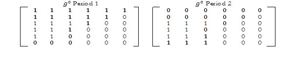
Let us use a poverty cutoff of 33% or two out of six dimensions. Increases and decreases are depicted in bold. Below we summarize ![]() ,
, ![]() and
and ![]() in two periods and their changes across two periods.
in two periods and their changes across two periods.

So in period two there are four kinds of changes affecting the dynamic subgroups as follows:
1) ![]() : persons 1 and 2 become non-poor (move out of or exit poverty)
: persons 1 and 2 become non-poor (move out of or exit poverty)
2) ![]() person 6 enters poverty.
person 6 enters poverty.
3) ![]() two kinds of changes occur
two kinds of changes occur
a. deprivations of ongoing poor persons 3 and 4 reduce by one deprivation each
b. deprivations of ongoing poor person 5 increases by one deprivation.
The descriptions and the decompositions of ![]() for the changes are in the following table.
for the changes are in the following table.
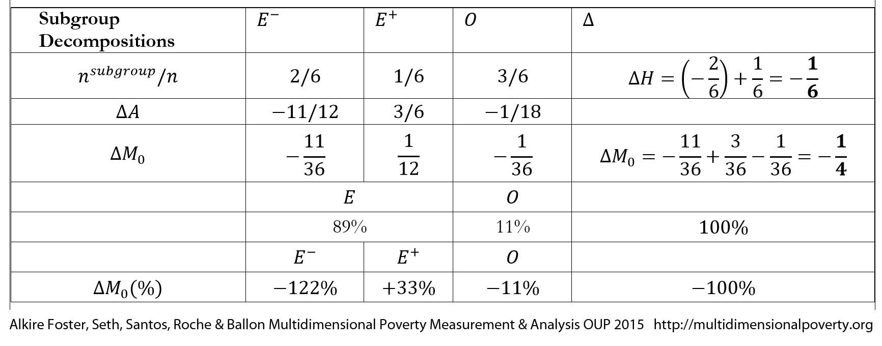
What is particularly interesting for policy is that we can notice that, in this example, 11% of the reduction in poverty was due to changes in intensity among the 50% of the population who stayed poor, that poverty was effectively increased 33% by the new entrant, but that this was more than compensated by those who exited poverty (–122%), because they initially had very high intensities. In this dramatic example, the poorest of the poor exited poverty, while the less poor experienced smaller reductions.
9.3.2 Decomposition by Incidence and Intensity for Cross-Sectional Data
The previous section explained the changes for a fixed population over time. To estimate that empirically requires panel data with data on the same persons in both periods which can be used to track their movement in and out of poverty. Yet analyses over time are often based on repeated cross-sectional data having independent samples that are statistically representative of the population under study, but that do not to track each specific observation over time. This section examines the decomposition of changes in ![]() for cross-sectional data.
for cross-sectional data.
With cross-sectional data, we cannot distinguish between the three groups identified above, nor can we isolate the intensity of those who move into or out of poverty. Observed values are only available for: ![]() and
and ![]() . Using these, it is categorically impossible to decompose
. Using these, it is categorically impossible to decompose ![]() with the empirical precision that panel data permits.
with the empirical precision that panel data permits.
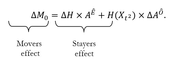
Nonetheless, if required one can move forward with some simplifications. Instead of three groups (![]() let us consider just two, which might be referred to (somewhat roughly) as movers and stayers. We define movers as the
let us consider just two, which might be referred to (somewhat roughly) as movers and stayers. We define movers as the ![]() people who reflect the net change in poverty levels across the two periods. Stayers are ongoing poor plus the proportion of previously poor people who were replaced by ‘new poor’, and total those who are poor in period 2
people who reflect the net change in poverty levels across the two periods. Stayers are ongoing poor plus the proportion of previously poor people who were replaced by ‘new poor’, and total those who are poor in period 2 ![]() . In considering only the ‘net’ change in headcount, one effectively permits the larger of
. In considering only the ‘net’ change in headcount, one effectively permits the larger of ![]() to dominate: if poverty rose nationally, it is the group who entered poverty who dominate; if poverty fell nationally, the group who exited poverty. The subordinate third group is allocated among the ongoing poor and the dominant group. For the remainder of this section we presume that both
to dominate: if poverty rose nationally, it is the group who entered poverty who dominate; if poverty fell nationally, the group who exited poverty. The subordinate third group is allocated among the ongoing poor and the dominant group. For the remainder of this section we presume that both ![]() and
and ![]() decreased overall. In this case,
decreased overall. In this case, ![]() . So
. So ![]() , and
, and ![]() =
=![]() . As is evident, this simplification is performed because empirical data exist in repeated cross-sections for
. As is evident, this simplification is performed because empirical data exist in repeated cross-sections for ![]() and
and ![]() .
.
Example: Suppose that 37% of people are ongoing poor, 3% enter poverty, 13% exit poverty, and 47% remain non-poor. Suppose the overall headcount ratio decreased by 10 percentage points, and the headcount ratio in period 2 is 40%, whereas in period 1 it was 50% (37%+13%). We now primarily consider two numbers: the headcount ratio in period 2 of 40% (interpreted broadly as ongoing poverty) and the change in headcount ratio of 10% (interpreted broadly as moving into/out of poverty). In doing so we are effectively permitting the ‘new poverty entrants’ to be considered as among the group in ongoing poverty in period 2 (37% + 3% = 40%). To balance this, we effectively replace 3% of those who exited poverty (13% – 3% = 10% =![]() ), and consider this slightly reduced group to be those who moved out of poverty. If poverty had increased overall, the swaps would be in the other direction.
), and consider this slightly reduced group to be those who moved out of poverty. If poverty had increased overall, the swaps would be in the other direction.
If poverty has reduced and there has not been a large influx of people into poverty, that is, if ![]() is presumed to be relatively small empirically, then this strategy would be likely to shed light on the relative intensity levels of those who moved out of poverty
is presumed to be relatively small empirically, then this strategy would be likely to shed light on the relative intensity levels of those who moved out of poverty ![]() , and the changes in intensity among those who remained poor
, and the changes in intensity among those who remained poor ![]() . If empirically
. If empirically ![]() is expected (from other sources of information) to be large, or if their intensity is expected to differ greatly from the average, this strategy is not advised.[16]
is expected (from other sources of information) to be large, or if their intensity is expected to differ greatly from the average, this strategy is not advised.[16]
Consider the intensity of the net population who exited poverty – under these simplifying assumptions reflected by the net change in headcount, denoted ![]() and the intensity change of the net ongoing poor, whom we will presume to be
and the intensity change of the net ongoing poor, whom we will presume to be ![]() , denoted
, denoted ![]() . The
. The ![]() can be decomposed according to these two groups. These decompositions can be interpreted as showing percentage of the change in
can be decomposed according to these two groups. These decompositions can be interpreted as showing percentage of the change in ![]() that can be attributed to those who moved out of poverty, versus the percentage of change which was mainly caused by a decrease in intensity among those who stayed poor. We use the terms movers and stayers to refer to these less precise dynamic subgroups in cross-sectional data analysis.
that can be attributed to those who moved out of poverty, versus the percentage of change which was mainly caused by a decrease in intensity among those who stayed poor. We use the terms movers and stayers to refer to these less precise dynamic subgroups in cross-sectional data analysis.
|
|
(9.16) |
Cross sectional data does not provide the intensity of either of those who stayed poor or of those who moved out of poverty. One way forward is to estimate these using existing data. First, identify the ![]() poor persons having the lowest intensity in the dataset (sampling weights applied), and use the average of these scores for
poor persons having the lowest intensity in the dataset (sampling weights applied), and use the average of these scores for ![]() then solve for Subsequently, identify the
then solve for Subsequently, identify the ![]() poor persons having the highest intensity in that dataset, and repeat the procedure. This will generate upper and lower estimates for
poor persons having the highest intensity in that dataset, and repeat the procedure. This will generate upper and lower estimates for ![]() and
and ![]() in a given dataset, which will provide an idea of the degree of uncertainty that different assumptions introduce. To estimate stricter upper and lower bounds it could be assumed that those moved out of poverty had an intensity score of the value of
in a given dataset, which will provide an idea of the degree of uncertainty that different assumptions introduce. To estimate stricter upper and lower bounds it could be assumed that those moved out of poverty had an intensity score of the value of ![]() (the theoretically minimum possible), and subsequently assume that their intensity was 100% (the theoretically maximum possible).[18]
(the theoretically minimum possible), and subsequently assume that their intensity was 100% (the theoretically maximum possible).[18]
Table 9.6 provides the empirical estimations for the upper and lower bounds for the same four countries discussed above plus Ethiopia. At the upper bound those who moved out of poverty could have had average intensities ranging from 59% in Peru (the least poor country) to 99% in Ethiopia or 100% in Senegal, according to the datasets. This in itself is interesting, as it shows that Rwanda—which is the poorest country of the four—had ‘movers’ with lower average deprivations than Ethiopa. Those who stayed poor would have had, in this case, small if any increases or decreases in intensity—less than four percentage points. At the lower bound, those who moved out of poverty could have had intensities from 33% in Peru and Senegal to 38% in Nepal, and intensity reductions among the ongoing poor could have ranged from 2% in Senegal to 13% in Nepal. At the upper bound (where we assume the poorest of the poor moved out of poverty), for Nepal, Rwanda and Peru, over 100% of the poverty reduction was due to the movers, because intensity among the ongoing poor would have had to increase (to create the observed ![]() ). At the lower bound, where the least poor people moved out of poverty, movers contributed 47–67% to
). At the lower bound, where the least poor people moved out of poverty, movers contributed 47–67% to ![]() . Senegal did not have a statistically significant reduction in poverty. Ethiopia provides a different example where the upper and lower bound are closer together and reductions in intensity among the ongoing poor would have contributed 31% to 73%.
. Senegal did not have a statistically significant reduction in poverty. Ethiopia provides a different example where the upper and lower bound are closer together and reductions in intensity among the ongoing poor would have contributed 31% to 73%.
Table 9.6 Decomposing the Change in ![]() by Dynamic Subgroups
by Dynamic Subgroups
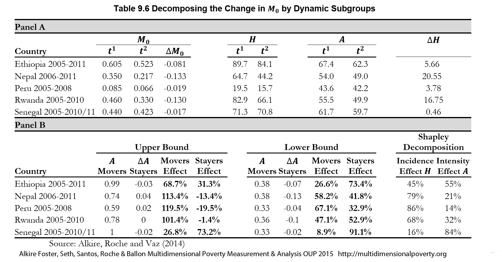 This empirical investigation shows that, when implemented with the mild assumptions that are required for cross-sectional data, the upper and lower bounds according to each country’s dataset are very wide apart. In reality, the relative contribution, of the ‘movers’ and ‘stayers’ to overall poverty reduction could vary anywhere in this range.
As the example shows, the empirical upper and lower bounds vary greatly across countries. In the case of Ethiopia, movers explain 27% to 69% of the changes in poverty, and stayers account for 31% to 73%. These boundaries do not permit us to assess whether the actual contribution from ‘movers’ was greater than or less than that of ‘stayers’. In Nepal and Peru the ‘movers’ probably contributed more than ‘stayers’ to poverty reduction, as in all cases their lowest effect is above 50%. Given these wide-ranging upper and lower bounds, empirically we are unable to answer questions such as whether the intensity of the ongoing poor decreased, or whether it was the barely poor or the deeply poor who moved out of poverty. While this can seem disappointing, for policy purposes, as Sen stresses, it may be better to be ‘vaguely right than precisely wrong’, and repeated cross-sectional data simply do not permit us, at this time, to bound ahead with precision.
9.3.3 Theoretical Incidence-Intensity Decompositions
Whereas monitoring and policy inputs must be based on empirical analyses, some research topics utilize theoretical analyses. This section introduces two theory-based approaches to decomposing changes in repeated cross-sectional data according to what we call ‘incidence’ and ‘intensity’. In each approach assumptions are made regarding the intensity of those who exit or remain poor. As we have already noted, the task implies some challenges because the empirical accuracy of the underlying assumptions is completely unknown, and as Table 9.6 showed, the actual range may be quite large. These techniques are thus offered in the spirit of academic inquiry.
For simplicity of notation, in this subsection, we denote the ![]() ,
, ![]() , and
, and ![]() for period
for period ![]() by
by ![]() ,
, ![]() and
and ![]() and that for period
and that for period ![]() by
by ![]() ,
, ![]() and
and ![]() . The first approach consists in the additive decomposition proposed by Apablaza and Yalonetzky (2013), which is illustrated in Panel A of Figure 9.2. Since
. The first approach consists in the additive decomposition proposed by Apablaza and Yalonetzky (2013), which is illustrated in Panel A of Figure 9.2. Since ![]() , they propose to decompose the change in
, they propose to decompose the change in ![]() by changes in its partial indices as follows
by changes in its partial indices as follows
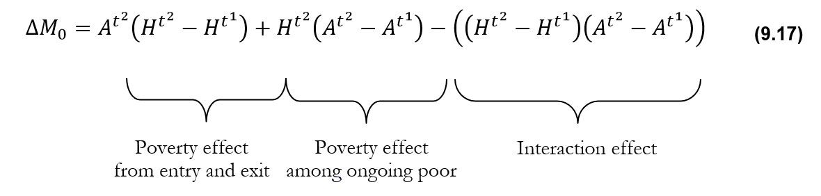 Note that the illustration in Figure 9.2 assumes reductions in
 ![]() ,
, ![]() , and
, and ![]() over time, but the graph can be adjusted to incorporate situations where they do not necessarily fall. This approach involves two assumptions. First, the intensity among those who left poverty is assumed to be the same as the average intensity in period
over time, but the graph can be adjusted to incorporate situations where they do not necessarily fall. This approach involves two assumptions. First, the intensity among those who left poverty is assumed to be the same as the average intensity in period ![]() . Second, the intensity change among the ongoing poor is assumed to equal the simple difference in intensities of the poor across the two periods. The decomposition is completed using an interaction term, as depicted in Panel A of Figure 9.2, below. This is indeed an additive decomposition of changes in the Adjusted Headcount Ratio
. Second, the intensity change among the ongoing poor is assumed to equal the simple difference in intensities of the poor across the two periods. The decomposition is completed using an interaction term, as depicted in Panel A of Figure 9.2, below. This is indeed an additive decomposition of changes in the Adjusted Headcount Ratio ![]() Apablaza and Yalonetzky interpret these changes as reflecting: (1) changes in the incidence of poverty
Apablaza and Yalonetzky interpret these changes as reflecting: (1) changes in the incidence of poverty ![]() , (2) changes in the intensity of poverty
, (2) changes in the intensity of poverty ![]() , and (3) a joint effect that is due to interaction between incidence and intensity (
, and (3) a joint effect that is due to interaction between incidence and intensity (![]() .
.
Figure 9.2 Theoretical Decompositions
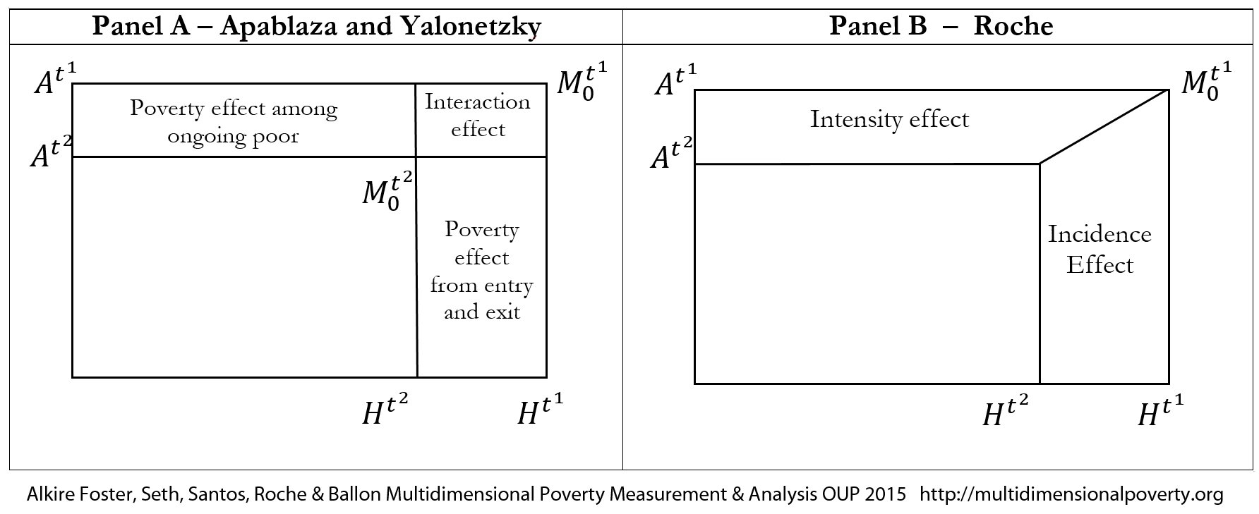 A second theoretical approach corresponds to a Shapley decomposition proposed by Roche (2013). This builds on Apablaza and Yalonetzky (2013) and performs a Shapley value decomposition following Shorrocks (1999).[19] It provides the marginal effect of changes in incidence and intensity as follows:
|
|
|
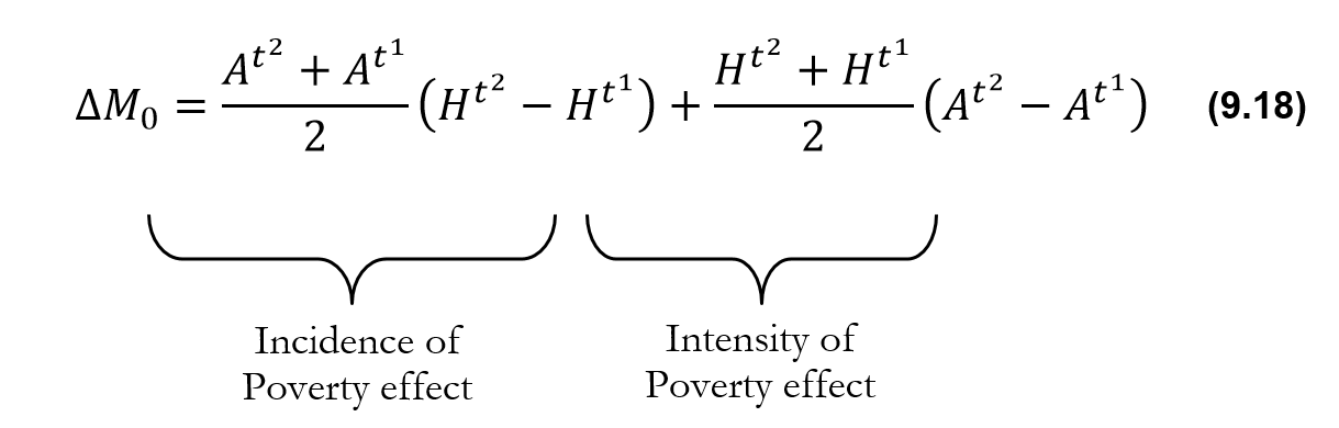
Panel B of Figure 9.2 illustrates Roche’s application of Shapley decompositions, which focuses on the marginal effect without the interaction effect. Roche’s proposal assumes that the intensity of those who exited poverty (our terms) is the average intensity of the two periods  , and calls this the ‘incidence effect’. He takes the other group as comprising the average headcount ratio between the two periods, and their change in intensity as the simple difference in intensities across the periods
  and describes this as the ‘intensity effect’.
Roche’s masterly presentation systematically applies Shapley decompositions to each step of dynamic analysis using the AF method. For example, if the underlying assumptions are transparently stated and accepted, the theoretically derived marginal contribution of changes in incidence and marginal contribution of changes in intensity can be expressed as a percentage of the overall change in ![]() so they both add to 100% and can be written as follows
so they both add to 100% and can be written as follows
|
|
(9.19) |
|
|
|
(9.20) |
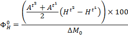
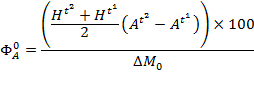
To address demographic shifts Roche follows a similar decomposition of change as that used in FGT unidimensional poverty measures (Ravallion and Huppi, 1991) and Shapely decompositions (Duclos and Araar 2006, Shorrocks 1999). This approach, presented in Equation (9.21), attribute demographic effects to the average population shares and subgroup ![]() ’s across time. Roche argues that, if the underlying assumptions are accepted, the overall change in poverty level can be broken down in two components: 1) changes due to intra-sectoral or within-group poverty effect, 2) changes due to demographic or inter-sectoral effect. So the overall change in the adjusted headcount between two periods respectively
’s across time. Roche argues that, if the underlying assumptions are accepted, the overall change in poverty level can be broken down in two components: 1) changes due to intra-sectoral or within-group poverty effect, 2) changes due to demographic or inter-sectoral effect. So the overall change in the adjusted headcount between two periods respectively![]() , could be expressed as follows
, could be expressed as follows
|
|
|
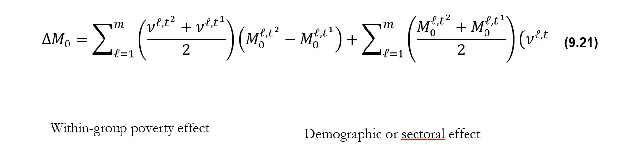
It is common to express the contribution of each factor as a proportion of the overall change, in which case equation (9.21) is divided throughout by ![]()
The last columns of Table 9.6 Panel B provide Shapley decompositions for the same five countries. We see that in all cases the Shapley decompositions lie, as anticipated, between the upper and lower bounds. The Shapley decompositions have the broad appeal of presenting point estimates that pinpoint the exact contribution of each partial index to changes in poverty, according to their underlying assumptions, and thus may be used in analyses when empirical accuracy is not required or the assumptions are independently verified. A full illustration of the Shapley decomposition methods using data on multidimensional child poverty in Bangladesh is given in Roche (2013).[20]
9.4 This Complementary Chronic Poverty with Multiple Time Periods
Panel datasets provide information on precisely the same individual or household at different periods of time. Good quality panel datasets are particularly rich and useful for analysing multidimensional poverty because their analysis provides policy-relevant insights that extend what time series data provide. For example, using panel data we can distinguish the deprivations experienced by the chronically poor from those experienced by the transitory poor and thus identify the combination of deprivations that trap people in long-term multidimensional poverty. Also, we can analyse the duration over which a person was deprived in each indicator—and the sequences by which their deprivation profile evolved. As section 9.3.1 showed, we can identify precisely the contributions to poverty reduction that were generated by changes entries and exits from poverty and by the ongoing poor.
The following section very briefly presents a counting-based class of chronic multidimensional poverty measures that use a triple-cutoff method of identifying who is poor. We give prominence here to the measure that can be estimated using ordinal data. The partial indices associated with the chronic multidimensional poverty methodology include the headcount ratio and intensity, as well as new indices related to the duration of poverty and of dimensional deprivation. We also present a linked measure of transient poverty. As in other sections, we presume that interested readers will master standard empirical and statistical techniques that are appropriate for studies using panel data, and apply these in the analyses of poverty transitions and chronic poverty here described.
The closing section on poverty transitions informally sketches revealing analyses that can be undertaken without generating a chronic poverty measure. Rather, people are identified as multidimensionally poor or non-poor in each period, then population subgroups are identified that have differing sequences of multidimensional poverty. For example, one group might include non-poor people who ‘fell’ into multidimensional poverty, a second might include multidimensionally poor people who ‘rose’ out of poverty, a third might contain those who were poor in all periods, and a fourth might contain those who ‘churned’ in and out of poverty across periods. Naturally the number of ‘dynamic subgroups’ depends upon the sample design, the number of waves of data and the precise definition of each group.
9.4.1 Chronic Poverty Measurement Using Panel Data
Multiple approaches to measuring chronic poverty in one dimension exist, many of which have implications for the measurement of chronic multidimensional poverty.[21] Alongside important qualitative work, multiple methodologies for measuring chronic multidimensional poverty have also been proposed.[22] This section combines the AF methodology with the counting-based approach to chronic poverty measurement proposed in Foster (2009), which has a dual-cutoff identification structure and aggregation method that are very similar to the AF method. Foster (2009) provides a methodology for measuring unidimensional chronic poverty in which each time period ![]() is equally weighted for all a
is equally weighted for all a![]() An
An ![]() matrix is constructed in which each entry takes a value of one if person
matrix is constructed in which each entry takes a value of one if person ![]() is identified as poor in period
is identified as poor in period ![]() and a value of 0 otherwise. A
and a value of 0 otherwise. A ![]() -dimensional ‘count’ vector is constructed in which each entry shows the number of periods in which person
-dimensional ‘count’ vector is constructed in which each entry shows the number of periods in which person ![]() was poor. A second time cutoff
was poor. A second time cutoff![]() is applied such that each person is identified as chronically poor if he or she has been poor in
is applied such that each person is identified as chronically poor if he or she has been poor in ![]() or more periods. Associated FGT indices and partial indices are then constructed from the relevant censored matrices.
or more periods. Associated FGT indices and partial indices are then constructed from the relevant censored matrices.
9.4.1.1 Order of Aggregation
This combined chronic multidimensional poverty measure applies three sets of cutoffs: deprivation cutoffs![]() , a multidimensional poverty cutoff
, a multidimensional poverty cutoff ![]() , and a duration cutoff
, and a duration cutoff ![]() . It is possible to analyse multidimensional poverty using panel data by combining the AF methodology and the Foster (2009) chronic poverty methods following two different orders of aggregation, which we call chronic deprivation or chronic poverty. These alternatives effectively interchange the order in which the poverty and duration cutoffs are applied. In both cases, we first apply a fixed set of deprivation cutoffs to the achievement matrix in each period.
. It is possible to analyse multidimensional poverty using panel data by combining the AF methodology and the Foster (2009) chronic poverty methods following two different orders of aggregation, which we call chronic deprivation or chronic poverty. These alternatives effectively interchange the order in which the poverty and duration cutoffs are applied. In both cases, we first apply a fixed set of deprivation cutoffs to the achievement matrix in each period.
In the chronic deprivation option (![]() before
before ![]() ), we first consider the duration of deprivation in each indicator for each person and then compute a multidimensional poverty measure which summarizes only those deprivations that have been experienced by the same person across
), we first consider the duration of deprivation in each indicator for each person and then compute a multidimensional poverty measure which summarizes only those deprivations that have been experienced by the same person across ![]() or more periods. This approach aggregates all ‘chronic’ deprivations into a multidimensional poverty index, regardless of the period in which those deprivations were experienced. This approach would provide complementary information that could enrich analyses of multidimensional poverty, but cannot be broken down by time period, nor does it show whether the deprivations were experienced simultaneously (Alkire, Apablaza, Chakravarty, and Yalonetzky 2014).
or more periods. This approach aggregates all ‘chronic’ deprivations into a multidimensional poverty index, regardless of the period in which those deprivations were experienced. This approach would provide complementary information that could enrich analyses of multidimensional poverty, but cannot be broken down by time period, nor does it show whether the deprivations were experienced simultaneously (Alkire, Apablaza, Chakravarty, and Yalonetzky 2014).
In the chronic multidimensional poverty option (![]() before
before ![]() ), we first identify each person as multidimensionally poor or non-poor in each period using the poverty cutoff
), we first identify each person as multidimensionally poor or non-poor in each period using the poverty cutoff![]() . We then count the periods in which each person experienced multidimensional poverty. We identify as chronically multidimensionally poor those persons who have experienced multidimensional poverty in
. We then count the periods in which each person experienced multidimensional poverty. We identify as chronically multidimensionally poor those persons who have experienced multidimensional poverty in ![]() or more periods.
or more periods.
9.4.1.2 Deprivation matrices
We observe achievements across ![]() dimensions for a set of
dimensions for a set of ![]() individuals at
individuals at ![]() different time points. Let
different time points. Let ![]() stand for the achievement in attribute
stand for the achievement in attribute ![]() of person
of person ![]() in period
in period ![]() , where
, where ![]() Let
Let ![]() denote a
denote a ![]() matrix whose elements reflect the dimensional achievements of the population in period
matrix whose elements reflect the dimensional achievements of the population in period ![]() . The deprivation cutoff vector
. The deprivation cutoff vector ![]() is fixed across periods. As before, a person is deprived with respect to deprivation
is fixed across periods. As before, a person is deprived with respect to deprivation ![]() in periods
in periods ![]() if
if ![]() and non-deprived otherwise. By applying the deprivation cutoffs to the achievement matrix for each period, we can construct the period-specific deprivation matrices
and non-deprived otherwise. By applying the deprivation cutoffs to the achievement matrix for each period, we can construct the period-specific deprivation matrices ![]() . For simplicity, this section uses the non-normalized or numbered weights notation across dimensions, such that
. For simplicity, this section uses the non-normalized or numbered weights notation across dimensions, such that ![]() Time periods are equally weighted. When achievement data are cardinal we can also construct normalized gap matrices
Time periods are equally weighted. When achievement data are cardinal we can also construct normalized gap matrices ![]() and squared gap matrices
and squared gap matrices ![]() or more generally, powered matrices of normalized deprivation gaps
or more generally, powered matrices of normalized deprivation gaps ![]() where
where ![]() . In a similar manner as previously, we generate the
. In a similar manner as previously, we generate the ![]() -dimensional
-dimensional ![]() column vector, which reflects the weighted sum of deprivations person
column vector, which reflects the weighted sum of deprivations person ![]() experiences in periods
experiences in periods ![]() .
.
9.4.1.3 Identification
To identify who is chronically multidimensionally poor we first construct an identification matrix. The same matrix can be used to identify the transient poor in each period and to create subgroups of those who exhibit distinct patterns of multidimensional poverty (for analysis of poverty transitions).
Identification Matrix
Let ![]() be an
be an ![]() identification matrix whose typical element
identification matrix whose typical element ![]() is one if person
is one if person ![]() is identified as multidimensionally poor in period
is identified as multidimensionally poor in period ![]() using the AF methodology, that is, using a poverty cutoff
using the AF methodology, that is, using a poverty cutoff ![]() which is fixed across periods, and 0 otherwise.
which is fixed across periods, and 0 otherwise.
The typical column ![]() reflects the identification status
reflects the identification status ![]() for the
for the ![]() th person in period
th person in period ![]() , whereas the typical row
, whereas the typical row ![]() displays the periods in which person
displays the periods in which person ![]() has been identified as multidimensionally poor (signified by an entry of 1) or non-poor (0). Thus we might equivalently consider each column of
has been identified as multidimensionally poor (signified by an entry of 1) or non-poor (0). Thus we might equivalently consider each column of ![]() to be an identification column vector for period
to be an identification column vector for period ![]() such that
such that ![]() if and only if person
if and only if person ![]() is multidimensionally poor in period
is multidimensionally poor in period ![]() according to the deprivation cutoffs
according to the deprivation cutoffs ![]() , weights
, weights ![]() , and poverty cutoff
, and poverty cutoff ![]() ; and
; and ![]() otherwise.
otherwise.
Episodes of Poverty Count Vector ![]()
From the ![]() matrix we construct the
matrix we construct the ![]() -dimensional column vector
-dimensional column vector ![]() whose
whose ![]() th element
th element ![]() =
= ![]() sums the elements of the corresponding row vector of
sums the elements of the corresponding row vector of ![]() and provides the total number of periods in which person
and provides the total number of periods in which person ![]() is poor, or the total episodes of poverty, as identified by poverty cutoff
is poor, or the total episodes of poverty, as identified by poverty cutoff ![]() . Naturally,
. Naturally, ![]() , that is, each person may have from 0 episodes of poverty to
, that is, each person may have from 0 episodes of poverty to ![]() episodes, the latter indicating that a person was poor in each of the
episodes, the latter indicating that a person was poor in each of the ![]() periods.
periods.
Chronic Multidimensional Poverty: Identification and Censoring
We apply the duration cutoff![]() where
where ![]() to the
to the ![]() vector in order identify the status of each person as chronically multidimensionally poor or not. We identify a person to be chronically multidimensionally poor if
vector in order identify the status of each person as chronically multidimensionally poor or not. We identify a person to be chronically multidimensionally poor if ![]() . That is, if they have experienced
. That is, if they have experienced ![]() or more periods in multidimensional poverty. A person is considered non-chronically poor if
or more periods in multidimensional poverty. A person is considered non-chronically poor if ![]() . We doubly censor the
. We doubly censor the ![]() vector such that it takes the value of 0 (non-chronically poor) if
vector such that it takes the value of 0 (non-chronically poor) if ![]() and takes the value of
and takes the value of ![]() otherwise. The notation
otherwise. The notation ![]() indicates the censored vector of poverty episodes—just as the notation
indicates the censored vector of poverty episodes—just as the notation ![]() indicated the censored deprivation count vector. Positive entries reflect the number of periods in which chronically poor people experienced poverty; entries of 0 mean that the person is not identified as chronically poor.
indicated the censored deprivation count vector. Positive entries reflect the number of periods in which chronically poor people experienced poverty; entries of 0 mean that the person is not identified as chronically poor.
Among the non-chronically poor, we could (as we will elaborate) identify two subgroups: the non-poor and the transient poor. A person is considered transiently poor if ![]() . And naturally a person for whom
. And naturally a person for whom ![]() , that is, who is non-poor in all periods, is considered non-poor.
, that is, who is non-poor in all periods, is considered non-poor.
An alternative but useful notation for the identification of chronic multidimensional poverty uses the identification function: we apply the identification function ![]() to censor the
to censor the ![]() matrix and the
matrix and the ![]() vector. The doubly censored
vector. The doubly censored ![]() matrix reflects solely those periods in poverty that are experienced by the chronically poor (censoring all periods of transient poverty) and is denoted by
matrix reflects solely those periods in poverty that are experienced by the chronically poor (censoring all periods of transient poverty) and is denoted by ![]() . After censoring, the typical element
. After censoring, the typical element ![]() is defined by
is defined by ![]() . The entry takes a value of
. The entry takes a value of ![]() if person
if person ![]() is chronically multidimensionally poor and 0 otherwise.
is chronically multidimensionally poor and 0 otherwise.
Censored ![]() Deprivation Matrices and Count Vector
Deprivation Matrices and Count Vector
To identify the censored headcounts, as well as the dimensional composition of poverty in each period, we censor the ![]() sets of
sets of ![]() deprivation matrices by applying the twin identification functions
deprivation matrices by applying the twin identification functions ![]() and
and ![]() . We denote the censored matrices by
. We denote the censored matrices by ![]() and the censored deprivation count vectors for each period
and the censored deprivation count vectors for each period ![]() .
.
Deprivation Duration Matrix
Finally, to summarize the overall dimensional deprivations of the poor, as well as the duration of these deprivations, it will be useful to create a duration matrix based on the censored deprivation matrices ![]() . Let
. Let ![]() be an
be an ![]() matrix whose typical element
matrix whose typical element ![]() provides the number of periods in which is chronically poor and is deprived in dimension
provides the number of periods in which is chronically poor and is deprived in dimension ![]() . Note that
. Note that ![]() We can use the duration matrix to obtain the deprivation-specific duration indices, which show the percentage of periods in which, on average, poor people were deprived in each indicator.
We can use the duration matrix to obtain the deprivation-specific duration indices, which show the percentage of periods in which, on average, poor people were deprived in each indicator.
9.4.1.4 Aggregation
The measure of chronic multidimensional poverty when some data are ordinal may be written as follows:
|
|
(9.22) |
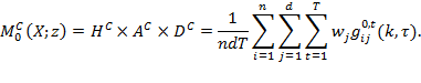
Thus the Adjusted Headcount Ratio of chronic multidimensional poverty![]() is the mean of the set of
is the mean of the set of ![]() deprivation matrices
deprivation matrices ![]() that have been censored of all deprivations of persons who are not chronically multidimensionally poor. Alternative notation for this measure can be found in Alkire, Apablaza, Chakravarty, and Yalonetzky (2014).
that have been censored of all deprivations of persons who are not chronically multidimensionally poor. Alternative notation for this measure can be found in Alkire, Apablaza, Chakravarty, and Yalonetzky (2014).
When data are cardinal, the ![]() class of measures are, like the AF class, the means of the respective powered matrices of normalized gaps.
class of measures are, like the AF class, the means of the respective powered matrices of normalized gaps.
|
|
(9.23) |
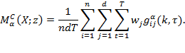
9.4.2 Properties
For chronic multidimensional poverty, as for multidimensional poverty, the specification of axioms is, in some cases, a joint restriction on the (triple-cutoff) identification and aggregation strategies and, hence, on the overall poverty methodology. The properties are now defined with respect to the chronically multidimensionally poor population. The class of measures present respects the key properties that were highlighted as providing policy relevance and practicality to the AF measures, such as subgroup consistency and decomposability, dimensional monotonicity, dimensional breakdown, and ordinality. In addition, this class of measures satisfies a form of time monotonicity as highlighted in Foster (2009) in the unidimensional case. The intuition is that if a person who is chronically poor becomes poor in an additional period, poverty rises.
A full definition of the properties that this chronic multidimensional poverty measure fulfils is provided in Alkire, Apablaza, Chakravarty, and Yalonetzky (2014). The methodology of multidimensional chronic poverty measurement fulfils the appropriately stated properties of anonymity, time anonymity, population replication invariance, chronic poverty focus, time focus, chronic normalization, chronic dimensional monotonicity, chronic weak monotonicity, time monotonicity, chronic monotonicity in thresholds, monotonicity in multidimensional poverty identifier, chronic duration monotonicity, chronic weak transfer, non-increasing chronic poverty under association-decreasing switch, and additive subgroup decomposability for all ![]() . The class of measures also satisfies chronic strong monotonicity for
. The class of measures also satisfies chronic strong monotonicity for ![]() and chronic strong transfer when
and chronic strong transfer when ![]() .
.
9.4.3 Consistent Partial Indices
Like ![]() , the chronic multidimensional poverty measure
, the chronic multidimensional poverty measure ![]() is the product of intuitive partial indices that convey meaningful information on different features of a society’s experience of chronic multidimensional poverty. In particular,
is the product of intuitive partial indices that convey meaningful information on different features of a society’s experience of chronic multidimensional poverty. In particular, ![]() where:
where:
· ![]() is the headcount ratio of chronic multidimensional poverty—the percentage of the population who are chronically multidimensionally poor according to
is the headcount ratio of chronic multidimensional poverty—the percentage of the population who are chronically multidimensionally poor according to ![]() and
and ![]() .
.
· ![]() is the average intensity of poverty among the chronically multidimensionally poor—the average share of weighted deprivations that chronically poor people experience in those periods in which they are multidimensionally poor.
is the average intensity of poverty among the chronically multidimensionally poor—the average share of weighted deprivations that chronically poor people experience in those periods in which they are multidimensionally poor.
· ![]() reflects the average duration of poverty among the chronically poor — the average share of
reflects the average duration of poverty among the chronically poor — the average share of ![]() periods in which they experience multidimensional poverty.
periods in which they experience multidimensional poverty.
These partial indices can also be calculated directly. In particular,
|
|
(9.24) |
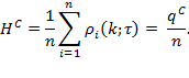
That is, the headcount ratio of chronic multidimensional poverty is the number of people who have been identified as chronically multidimensionally poor divided by the total population. We denote the number of chronically multidimensionally poor people by ![]()
The intensity of chronic multidimensional poverty is the sum of the weighted deprivation scores of all poor people over all time periods, divided by the number of dimensions times the total number of people who are poor in each period summed across periods. Note that ![]()
|
|
(9.25) |
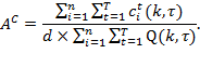
The average duration of chronic multidimensional poverty—the percentage of periods on average in which the chronically person was poor—can be easily assessed using the ![]() vector.
vector.
|
|
(9.26) |
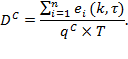
The duration is the sum of the total number of periods in which the chronically poor experience multidimensional poverty, divided by the number of periods and the number of chronically poor. Note that ![]() Box 9.2 illustrates these with a simple example.
Box 9.2 illustrates these with a simple example.
Box 9.2 Computing Incidence and Duration of Chronic Poverty
Consider three people and four periods, with ![]() = 2.
= 2.
Person 1 is multidimensionally poor in period 1
Person 2 is multidimensionally poor in periods 2, 3, and 4
Person 3 is multidimensionally poor in periods 1, 2, 3, and 4
Two people are chronically poor because they experience multidimensional poverty in ![]() = 2 or more periods. So the percentage of people identified as chronically poor
= 2 or more periods. So the percentage of people identified as chronically poor ![]() is 67%.
is 67%.
In this case, the vector ![]() =(0,3,4);
=(0,3,4); ![]() = 2 and our duration index is
= 2 and our duration index is![]() . That is, on average, chronically poor persons are poor during 87.5% of the time periods.
. That is, on average, chronically poor persons are poor during 87.5% of the time periods.
9.4.3.1 Dimensional Indices
For chronic multidimensional poverty, it is possible and useful to generate the standard dimensional indicators for each period: the censored headcount and percentage contribution. It is also possible and useful to generate the period-specific Adjusted Headcount Ratio (![]() ), headcount ratio (
), headcount ratio (![]() ), and intensity (
), and intensity (![]() ) figures, which are different from, but can be consistently related to, the chronic poverty headcount and intensity values presented in 9.4.3. Finally, and of tremendous use, it is possible to present the average duration of deprivation in each dimension and to relate this directly to the overall duration of chronic poverty. Box 9.3 presents the intuition of this set of consistent indices; for their precise definition see Alkire, Apablaza, Chakravarty, and Yalonetzky (2014).
) figures, which are different from, but can be consistently related to, the chronic poverty headcount and intensity values presented in 9.4.3. Finally, and of tremendous use, it is possible to present the average duration of deprivation in each dimension and to relate this directly to the overall duration of chronic poverty. Box 9.3 presents the intuition of this set of consistent indices; for their precise definition see Alkire, Apablaza, Chakravarty, and Yalonetzky (2014).
Box 9.3 Computing Incidence and Duration of Chronic Poverty
Cross-period indices reflecting chronic poverty:
![]() : Adjusted Headcount Ratio of chronic multidimensional poverty
: Adjusted Headcount Ratio of chronic multidimensional poverty
![]() : Headcount ratio, showing the percentage of the population who are chronically poor
: Headcount ratio, showing the percentage of the population who are chronically poor
![]() : Intensity, showing the average percentage of deprivations experienced by the chronically multidimensionally poor in those periods in which they are poor
: Intensity, showing the average percentage of deprivations experienced by the chronically multidimensionally poor in those periods in which they are poor
![]() : Average duration of chronic poverty, expressed as a percentage of time periods
: Average duration of chronic poverty, expressed as a percentage of time periods
![]() : Average censored headcount of dimension
: Average censored headcount of dimension ![]() among the chronically poor in all periods in which they are poor and are deprived in dimension
among the chronically poor in all periods in which they are poor and are deprived in dimension ![]()
![]() : Average duration of deprivation in dimension
: Average duration of deprivation in dimension ![]() among the chronically poor, expressed as a percentage of time periods
among the chronically poor, expressed as a percentage of time periods
![]() : Percentage contribution of dimension
: Percentage contribution of dimension ![]() to the deprivations of the chronically poor.
to the deprivations of the chronically poor.
Single-period indices reflecting the profiles of the chronic poor in that particular period of poverty:
![]() : Headcount ratio, showing the percentage of the population who are chronically poor in period
: Headcount ratio, showing the percentage of the population who are chronically poor in period ![]()
![]() : Intensity, showing the average percentage of deprivations experienced by the chronically multidimensionally poor in period
: Intensity, showing the average percentage of deprivations experienced by the chronically multidimensionally poor in period ![]()
![]() : Censored headcount of dimension
: Censored headcount of dimension ![]() among the chronically poor in period
among the chronically poor in period ![]()
![]() : Percentage contribution of dimension
: Percentage contribution of dimension ![]() to the deprivations of the chronically poor in period
to the deprivations of the chronically poor in period ![]() .
.
Cross-period averages of the unidimensional indices can also be constructed, such as ![]() and
and ![]() and analysed in conjunction with the relevant duration measure.
and analysed in conjunction with the relevant duration measure.
9.4.3.2 Censored Headcount Ratios
The censored headcount ratios for each period ![]() are constructed as the mean of the dimensional column vector for each period and represent the proportion of people who are chronically poor in time period
are constructed as the mean of the dimensional column vector for each period and represent the proportion of people who are chronically poor in time period ![]() and are deprived in dimension
and are deprived in dimension ![]() :
:
|
|
(9.27) |
We can also describe the average censored headcount ratios of chronic multidimensional poverty across ![]() periods in each dimension as simply the mean of the censored headcounts in each period:
periods in each dimension as simply the mean of the censored headcounts in each period:
|
|
(9.28) |
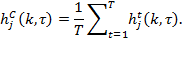
The Adjusted Headcount Ratio of chronic multidimensional poverty across all periods is simply the mean of the average weighted censored headcount ratios:
|
|
(9.29) |
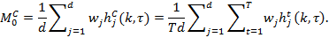
9.4.3.3 Percentage Contributions of Dimension
The percentage contributions show the (weighted) composition of chronic multidimensional poverty in each period and across periods.
We may seek an overview of the dimensional composition of poverty across all periods. The total percentage contribution of each dimension to chronic poverty across all periods is given by
|
|
(9.30) |
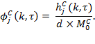
We may also be interested in analysing the percentage contributions of each dimension across various periods and thus in comparing the percentage contributions of dimensions across periods. The total percentage contribution in period ![]() is
is
|
|
(9.31) |
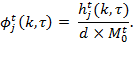
9.4.3.4 Censored Dimensional Duration
We are also able to construct a new set of statistics that provide more detail regarding the duration of dimensional deprivations among the chronically poor. We use the ![]() deprivation duration matrix
deprivation duration matrix ![]() , constructed in 9.4.1.3, in which each entry reflects the number of periods in which person
, constructed in 9.4.1.3, in which each entry reflects the number of periods in which person ![]() was chronically poor (by
was chronically poor (by ![]() and
and ![]() ) and was deprived in dimension
) and was deprived in dimension ![]() . Recall that for the chronically poor,
. Recall that for the chronically poor, ![]() in each dimension. The value of
in each dimension. The value of ![]() is, naturally, 0 for non-poor persons in all dimensions. Thus the matrix will have a positive entry for
is, naturally, 0 for non-poor persons in all dimensions. Thus the matrix will have a positive entry for ![]() persons and an entry of 0 for all persons who were never chronically poor.
persons and an entry of 0 for all persons who were never chronically poor.
For each dimension we can then define a dimensional duration index for dimension ![]() as follows
as follows
|
|
(9.32) |
The value of ![]() provides the percentage of periods in which the chronically poor were deprived in dimension
provides the percentage of periods in which the chronically poor were deprived in dimension ![]() on average.
on average.
The relationship between the mean across all ![]() and the chronic multidimensional poverty figure provided earlier is also elementary
and the chronic multidimensional poverty figure provided earlier is also elementary
|
|
(9.33) |
and
|
|
(9.34) |
9.4.3.5 Period-Specific Partial Indices
From the ![]() censored identification matrix
censored identification matrix ![]() we can also compute the period-specific headcounts of chronic multidimensional poverty. The headcount
we can also compute the period-specific headcounts of chronic multidimensional poverty. The headcount ![]() for period
for period ![]() is the mean of the column vector of
is the mean of the column vector of ![]() for period
for period ![]() . The average headcount across all periods is
. The average headcount across all periods is![]() . The average headcount across all periods and the chronic multidimensional poverty headcount are related by the average duration of poverty thus:
. The average headcount across all periods and the chronic multidimensional poverty headcount are related by the average duration of poverty thus:
|
|
(9.35) |

Similarly,
|
|
(9.36) |

and
|
|
(9.37) |
9.4.3.6 Illustration using Chilean CASEN
We present an example in Table 9.7 using three variables: schooling, overcrowding, and income in Chile’s CASEN (Encuesta de Caracterización Socioeconómica Nacional) dataset for three periods: 1996, 2001, and 2006. The table reports the Adjusted Headcount Ratio of chronic multidimensional poverty (![]() ) and its three partial indices: the headcount ratio (
) and its three partial indices: the headcount ratio (![]() ), the average chronic intensity (
), the average chronic intensity (![]() ) and the average duration (
) and the average duration (![]() ) for three poverty cutoffs
) for three poverty cutoffs ![]() and three different duration cutoffs
and three different duration cutoffs ![]() . All dimensions and periods are equally weighted for both identification and aggregation. When
. All dimensions and periods are equally weighted for both identification and aggregation. When ![]() and
and ![]() , the identification follows a double union approach. In this case, 49% of people are identified as chronically multidimensionally poor. However, a double-union approach does not appear to capture people who are either chronically or multidimensionally poor in any meaningful sense.
, the identification follows a double union approach. In this case, 49% of people are identified as chronically multidimensionally poor. However, a double-union approach does not appear to capture people who are either chronically or multidimensionally poor in any meaningful sense.
Table 9.7 Cardinal Illustration with Relevant Values of ![]() and
and ![]()
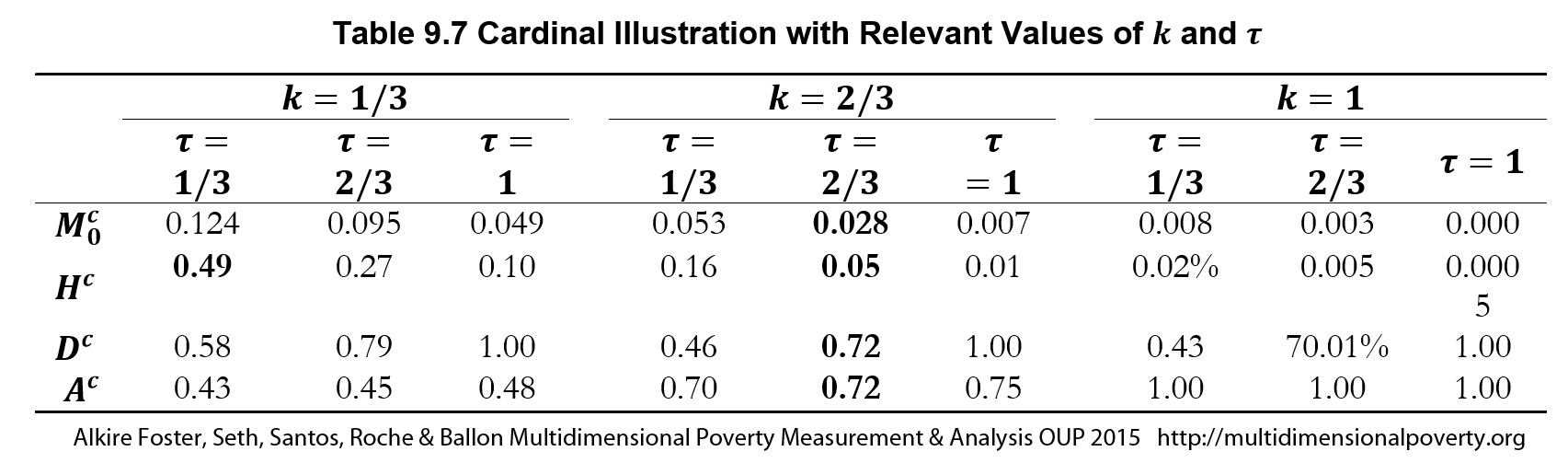 We thus consider the cutoffs where
 ![]() . In this situation, 5% of people are chronically multidimensionally poor. The average chronic intensity is 72%, meaning that people experience deprivations in 72% of dimensions in the periods in which they are poor. The average chronic duration is 72% also, meaning that the average poor person is deprived in 72% of the three periods. The overall chronic Adjusted Headcount Ratio of 0.028 shows that Chile’s population experiences only 2.8% of the deprivations it could possibly experience. All possible deprivations occur if all people are multidimensionally poor in all dimensions, and in all periods.
. In this situation, 5% of people are chronically multidimensionally poor. The average chronic intensity is 72%, meaning that people experience deprivations in 72% of dimensions in the periods in which they are poor. The average chronic duration is 72% also, meaning that the average poor person is deprived in 72% of the three periods. The overall chronic Adjusted Headcount Ratio of 0.028 shows that Chile’s population experiences only 2.8% of the deprivations it could possibly experience. All possible deprivations occur if all people are multidimensionally poor in all dimensions, and in all periods.
9.4.4 Poverty Transitions Using Panel Data
Using the identification matrix and the associated doubly censored deprivation matrices that have been constructed above, it is also possible to analyse poverty transitions. Comparisons can be undertaken – for example, between subgroups experiencing different dynamic patterns of multidimensional poverty – to ascertain different policy sequences or entry points that might have greater efficacy in eradicating multidimensional poverty. This section very briefly describes the construction of dynamic subgroups and some of the descriptive analyses that can be undertaken.
9.4.4.1 Constructing Dynamic Subgroups
The chronic multidimensional poverty measures constructed previously respect the property of subgroup consistency and subgroup decomposability; thus, they can be decomposed by any population subgroup for which the data are arguably representative. In addition, it can be particularly useful to describe multidimensional poverty for what we earlier called ‘dynamic subgroups’ – the definition of which can be extended when panel data cover more than two periods.
By ‘dynamic subgroups’, we mean population subgroups that experience different patterns of multidimensional poverty over time. These include the groups mentioned in section 9.3.1 who exited poverty (1,0), entered poverty (0,1), or were in ongoing poverty (1,1). The possible patterns will vary according to the number of waves in the sample as well as the observed patterns in the dataset. With three waves, there are four basic groups: falling—people who were non-poor and became multidimensionally poor; rising—people who were multidimensionally poor and exited poverty; churning—people who both enter and exit multidimensional poverty in different periods, and long-term—people who remain multidimensionally poor continuously.[23]
The dynamic subgroups are formed by considering the ![]() identification matrix
identification matrix ![]() . Note that we use the matrix that is censored by the poverty cutoff
. Note that we use the matrix that is censored by the poverty cutoff ![]() but we do not, in this section on poverty transitions, apply the duration cutoff. Consider a matrix of four persons and three periods in which each person experiences one of the four categories mentioned above. Recall that an entry of one indicates that person
but we do not, in this section on poverty transitions, apply the duration cutoff. Consider a matrix of four persons and three periods in which each person experiences one of the four categories mentioned above. Recall that an entry of one indicates that person ![]() is multidimensionally poor in period
is multidimensionally poor in period ![]() and a 0 indicates they are non-poor.
and a 0 indicates they are non-poor.
Falling: 0 0 1 (and 0 1 1)
Rising: 1 0 0 (and 1 1 0)
Churning: 1 0 1 (and 0 1 0)
Long-term: 1 1 1
For more than three periods, additional categories can be formed. Note that the categories can and must be mutually exhaustive. Each person who is multidimensionally poor in any period (whether chronically or transiently poor) can be categorized into one of these four groups.
9.4.4.2 Descriptive Analyses
Having decomposed the population into the non-poor and these (or additional) dynamic subgroups of the population, it can be useful to provide the standard partial indices for each subgroup, both per period and across all three periods:
· ![]() ,
, ![]() , and
, and ![]() (and standard errors);
(and standard errors);
· Percentage composition of poverty by dimension (often revealing) and censored headcounts;
· Intensity profiles across the poor (or inequality among the poor—see section 9.1).
It can also be useful to provide details regarding the sequences of evolution. For example, from the ![]() matrix, isolate the subgroup of the poor who ‘fell into’ poverty between period 1 and period 2 (that is, whose entries are 0,1 for the respective periods
matrix, isolate the subgroup of the poor who ‘fell into’ poverty between period 1 and period 2 (that is, whose entries are 0,1 for the respective periods ![]() and
and ![]() .). Compare their evolution with those who stayed poor (1,1) and those who stayed non-poor (0,0), in the following ways:
.). Compare their evolution with those who stayed poor (1,1) and those who stayed non-poor (0,0), in the following ways:
· At the individual level, compare the raw headcount in period 1 with the raw headcount in period 2.
· Identify the dimensions in which deprivations were (a) experienced in both periods, (b) only experienced in period 1, and (c) only experienced in period 2.
· Summarize the results, if relevant and legitimate, further decomposing the population into relevant subgroups whose compositional changes follow different patterns.
· Repeat for each adjacent pair of periods. Analyse whether the patterns are stable or differ across different adjacent periods.
Bibliography
Aaberge, R. and Peluso, E. (2012). ‘A Counting Approach for Measuring Multidimensional Deprivation.’ Statistics Norway Discussion paper 700.
Addison T., Hulme, D., and Kanbur R. (2009). Poverty Dynamics-Interdisciplinary Perspectives. OUP.
Alkire et al. (2014b): Alkire, S., Apablaza, M., Chakravarty, S., and Yalonetzky, G. (2014). ‘Measuring Chronic Multidimensional Poverty: A Counting Approach’. OPHI Working Paper 75, Oxford University.
Alkire, S. and Foster, J. (2011a). ‘Counting and Multidimensional Poverty Measurement’. Journal of Public Economics, 95(7–8): 476–487.
Alkire, S. and Foster, J. E. (2013). ‘Evaluating Dimensional and Distributional Contributions to Multidimensional Poverty’. OPHI: Mimeo.
Alkire, S. and Roche, J. M. (2013). ‘How Multidimensional Poverty Went Down: Dynamics and Comparisons?’. OPHI Briefing 16.
Alkire, S. and Seth, S. (2013b). ‘Multidimensional Poverty Reduction in India between 1999 and 2006: Where and How?’ OPHI Working Paper 60, Oxford University.
Alkire, S., Roche, J. M., and Seth S. (2011). ‘Sub-national Disparities and Inter-temporal Evolution of Multidimensional Poverty across Developing Countries’. OPHI Research in Progress 32a, Oxford University.
Alkire, S., Roche, J. M., and Seth S. (2013). ‘The Global Multidimensional Poverty Index 2013’. OPHI Briefing 13.
Alkire, S., Roche, J. M., and Vaz, A. (2014). ‘How Countries Reduce Multidimensional Poverty: A Disaggregated Analysis’. OPHI Working Paper 76, Oxford University.
Apablaza, M. and Yalonetzky, G. (2013) ‘Decomposing Multidimensional Poverty Dynamics’. Young Lives Working Paper 101.
Atkinson, A. B. and Bourguignon, F. (1982). ‘The Comparison of Multi-dimensioned Distributions of Economic Status’. Review of Economic Studies, 49(2): 183–201.
Baluch B. and Masset, E. (2003). ‘Do Monetary and Non-monetary Indicators Tell the Same Story about Chronic Poverty? A study of Vietnam in the 1990s’. World Development, 31(3): 441–453.
Bossert, W., Ceriani L., Chakravarty, S. R., and D’Ambrosio, C. (2012). ‘Intertemporal Material Deprivation’. CIREQ Cahier 07-2012.
Bossert, W., Chakravarty, S., and D’Ambrosio, C. (2013) ‘Multidimensional Poverty and Material Deprivation With Discrete Data’. Review of Income and Wealth, 59(1): 29–43.
Bourguignon, F., and Chakravarty, S. R. (2003). ‘The Measurement of Multidimensional Poverty’. Journal of Economic Inequality, 1(1): 25–49.
Calvo C. and Dercon, S. (2013). ‘Vulnerability to Individual and Aggregate Poverty’. Social Choice and Welfare 41(4): 721–740.
Calvo, C. (2008). ‘Vulnerability to Multidimensional Poverty: Peru, 1998–2002’. World Development 36(6): 1011–1020.
Chakravarty et al. (1998): Chakravarty, S. R., Mukherjee, D., and Ranade, R. R. (1998). ‘On the Family of Subgroup and Factor Decomposability Measures of Multidimensional Poverty’, in D. J. Slottje (ed.), Research on Economic Inequality 8. JAI Press, 175–194.
Chakravarty, S. R. (1983b). ‘A New Index of Poverty’. Mathematical Social Sciences, 6(3): 307-313.
Chakravarty, S. R. (2001). ‘The Variance as a Subgroup Decomposable Measure of Inequality’. Social Indicators Research, 53(1): 79–95.
Chakravarty, S. R. and D’Ambrosio, C. (2006). ‘The Measurement of Social Exclusion’. Review of Income and Wealth, 52(3): 377–398.
Chantreuil, F. and Trannoy, A. (2011). ‘Inequality Decomposition Values.’ Annals of Economics and Statistics, 101/102: 13-36.
Chantreuil, F. and Trannoy, A. (2013). ‘Inequality Decomposition Values: The Trade-off between Marginality and Efficiency,’ Journal of Economic Inequality, 11(1), 83-98.
Clark, C. R., Hemming, R., and Ulph, D. (1981). ‘On Indices for the Measurement of Poverty’. Economic Journal, 91(362): 515–526.
Datt, G. (2013). ‘Making Every Dimension Count: Multidimensional Poverty without the “Dual Cut Off”’. Monash Economics Working Papers 32–13.
Dercon, S. and Shapiro, J. (2007). ‘Moving On, Staying Behind, Getting Lost: Lessons on Poverty Mobility from Longitudinal Data’, in D. Narayan and P. Petesch (eds.), Moving out of Poverty, Vol. 1. World Bank, 77–126.
Duclos, J.-Y. and Araar, A. (2006). Poverty and Equity: Measurement, Policy and Estimation with DAD. Springer.
Foster J. and Santos M. E. (2013). ‘Measuring Chronic Poverty’, in G. Betti and A. Lemmi (eds.), Poverty and Social Exclusion: New Methods of Analysis. Routledge, 143–165.
Foster J., Greer, J., and Thorbecke, E. (1984). ‘A Class of Decomposable Poverty Measures’. Econometrica, 52(3): 761–766.
Foster, J. (2009). ‘A Class of Chronic Poverty Measures’, in T. Addison, Hulme, D., and R. Kanbur (eds.), Poverty Dynamics: Interdisciplinary Perspectives. OUP, 59–76.
Foster, J. E. and Sen, A. K. (1997). ‘On Economic Inequality after a Quarter Century’, an annexe to A. Sen, On Economic Inequality. OUP, 107–220.
Gordon et al. (2003) : Gordon, D., Nandy, S., Pantazis, Pemberton, S., and Townsend, P. (2003). Child Poverty in the Developing World. The Policy Press.
Gradín, C., del Rio, C., and Canto, O. (2012). ‘Measuring Poverty Accounting for Time’. Review of Income and Wealth, 58(2): 330–54.
Hoy, M. and Zheng, B. (2011). ‘Measuring Lifetime Poverty’. Journal of Economic Theory, 146(6): 2544–2562.
Hulme, D. and Shepherd, A. (2003). ‘Conceptualizing Chronic Poverty’. World Development, 31(3): 403–423.
Hulme, D., Moore, K., and Shepherd, A. (2001). ‘Chronic Poverty: Meanings and Analytical Frameworks’. CPRC Working Paper 2.
Jalan, J. and Ravallion, M. (1998). ‘Transient Poverty in Post-reform Rural China’. Journal of Comparative Economics, 26: 338–357.
Kolm, S. C. (1977). ‘Multidimensional Egalitarianisms’. The Quarterly Journal of Economics, 91(1): 1–13.
Maasoumi, E. and Lugo, M. A. (2008). ‘The Information Basis of Multivariate Poverty Assessments’, in N. Kakwani and J. Silber. (eds.), Quantitative Approaches to Multidimensional Poverty Measurement. Palgrave Macmillan: 1–29.
McKay, A. and Lawson, D. (2003). ‘Assessing the Extent and Nature of Chronic Poverty in Low Income Countries: Issues and Evidence’. World Development 31(3): 425–439.
Morduch, J. and Sinclair, T. (1998). Rethinking Inequality Decomposition, with Evidence from Rural China. Mimeo.
Narayan, D. and Petesch, P. (eds.). (2007). Moving out of Poverty: Cross-Disciplinary Perspectives on Mobility, Vol. 1. World Bank Publications.
Nicholas, A. and Ray, R. (2012). ‘Duration and Persistence in Multidimensional Deprivation: Methodology and Australian Application’. Economic Record 88(280): 106–126.
Nicholas, A., Ray, R., and Sinha, K. (2013). ‘A Dynamic Multidimensional Measure of Poverty’. Discussion Paper 25/13, Monash University, Melbourne.
Porter, C. and Quinn, N. (2013). ‘Measuring Intertemporal Poverty: Policy Options for the Poverty Analyst’, in G. Betti and A. Lemmi (eds.), Poverty and Social Exclusion: New Methods of Analysis. Routledge, 166–193.
Ravallion, M. and M. Huppi. (1991). ‘Measuring Changes in Poverty: A Methodological Case Study of Indonesia during an Adjustment Period’. World Bank Economic Review, 5(1): 57–82.
Rippin, N. (2012). Considerations of Efficiency and Distributive Justice in Multidimensional Poverty Measurement. PhD Dissertation, Georg-August-Universität Göttingen.
Roche, J. M. (2013). ‘Monitoring Progress in Child Poverty Reduction: Methodological Insights and Illustration to the Case Study of Bangladesh’. Social Indicators Research 112(2): 363–390.
Sen, A. (1976). ‘Poverty: An Ordinal Approach to Measurement’. Econometrica, 44(2): 219–231.
Seth, S. and Alkire, S. (2014a). ‘Measuring and Decomposing Inequality among the Multidimensionally Poor using Ordinal Variables: A Counting Approach’. OPHI Working paper 68, Oxford University.
Seth, S. and Alkire, S. (2014b). ‘Did Poverty Reduction Reach the Poorest of the Poor? Assessment Methods in the Counting Approach’. OPHI Working Paper 77, Oxford University.
Shorrocks, A. (1999) ‘Decomposition Procedures for Distributional Analysis: A Unified Framework Based on the Shapley Value’. Journal of Economic Inequality, 1–28.
Shorrocks, A. F. (1995). 'Revisiting the Sen Poverty Index'. Econometrica, 63(5): 1225–1230.
Silber, J. and Yalonetzky, G. (2014). ‘Measuring Multidimensional Deprivation with Dichotomized and Ordinal Variables’, in G. Betti and A. Lemmi (eds.), Poverty and Social Exclusion: New Methods of Analysis. Routledge, ch. 2.
Stewart, F. (2010). Horizontal Inequalities and Conflict. Palgrave Macmillan.
Thon, D. (1979). ‘On Measuring Poverty’. Review of Income and Wealth, 25: 429–440.
Tsui, K. (2002). ‘Multidimensional Poverty Indices’. Social Choice and Welfare 19(1): 69–93.
[1] For inequality-adjusted poverty measures in the unidimensional context, see Thon (1979), Clark, Hemming, and Ulph (1981), Chakravarty (1983b), Foster, Greer, and Thorbecke (1984), and Shorrocks (1995). For inequality-adjusted multidimensional poverty measures, i.e., those that satisfy transfer and/or strict rearrangement properties, see section section 3.6.
[2] This section summarizes these two papers.
[3] In order to say that one multidimensional distribution is more equal than another, each must be smoothed using the same bistochastic matrix.
[4] See Sen (1976) and Foster and Sen (1997).
[5] Bourguignon and Chakravarty (2003) and Datt (2013) also propose a similar class of indices but using a union identification criterion.
[6] We have already shown that our multidimensional measure ![]() satisfies weak transfer, the first type of transfer property, for
satisfies weak transfer, the first type of transfer property, for ![]() and the second type of transfer property, weak rearrangement, for
and the second type of transfer property, weak rearrangement, for ![]() . Chakravarty, Mukherjee, and Ranade (1998), Tsui (2002), Bourguignon and Chakravarty (2003), Chakravarty and D’Ambrosio (2006), Maasoumi and Lugo (2008), Aaberge and Peluso (2012), Bossert, Chakravarty, and D’Ambrosio (2013), and Silber and Yalonetzky (2014).
. Chakravarty, Mukherjee, and Ranade (1998), Tsui (2002), Bourguignon and Chakravarty (2003), Chakravarty and D’Ambrosio (2006), Maasoumi and Lugo (2008), Aaberge and Peluso (2012), Bossert, Chakravarty, and D’Ambrosio (2013), and Silber and Yalonetzky (2014).
[7] For empirical examples, see Alkire, Roche, and Seth (2013), who compare countries across four gradients of poverty.
[8] There are many variations. For example, if data are relatively accurate one might consider inequality using the uncensored deprivation score vector ![]() , and alternatively if one only wishes to capture inequality within some subgroup
, and alternatively if one only wishes to capture inequality within some subgroup![]() , then
, then ![]() and
and ![]() .
.
[9] If one is interested in decomposing (9.6) into within and between group components, then the total within-group inequality term can be computed as ![]() and the total between-group inequality term can be computed as
and the total between-group inequality term can be computed as ![]() , where
, where ![]() the intensity of each subgroup
the intensity of each subgroup ![]() such that
such that ![]() and
and ![]() is the share of all poor in subgroup
is the share of all poor in subgroup ![]() .
.
[10] This section draws on Alkire, Roche, and Vaz (2014).
[11] Tables of the absolute levels and absolute rates of change make this feature visible; reporting the relative rate of change underscores this more precisely.
[12] For small samples, one needs to conduct hypothesis tests using the Student-t distribution which are very similar to the hypothesis tests described in Chapter 8 that use the Standard Normal distribution.
[13] Normative issues in assigning weights were discussed in details in Chapter 6.
[14] Comparisons of reductions in both raw and censored headcounts may be supplemented by information on migration, demographic shifts, or exogenous shocks, for example.
[15] Suitable adjustments can be made for demographic shifts when the population is not fixed across two periods.
[16]The corresponding considerations apply if poverty has increased and ![]() is expected to be small
is expected to be small
[17] Naturally it is also possible to create estimates for ![]() where the upper bound was the overall change in intensity, and the lower bound was zero, and solve for
where the upper bound was the overall change in intensity, and the lower bound was zero, and solve for ![]() . However this would not permit an increase in intensity (which would happen if the barely poor left poverty and the others stayed the same, for example), nor for an even stronger reduction in intensity. For example, in the example in Table 9.2, Nepal’s A reduced by five percentage points, whereas in our upper bound, intensity among the ‘stayers’ increased by 4% and in the lower bound it decreased by 13%.
. However this would not permit an increase in intensity (which would happen if the barely poor left poverty and the others stayed the same, for example), nor for an even stronger reduction in intensity. For example, in the example in Table 9.2, Nepal’s A reduced by five percentage points, whereas in our upper bound, intensity among the ‘stayers’ increased by 4% and in the lower bound it decreased by 13%.
[18] These bounds are theoretically possible lower and upper bounds. Further research using panel datasets is required to investigate the likelihood of these bounds.
[19] The Shapley value decomposition was initially applied to decomposition of income inequality by Chantreuil and Trannoy (2011, 2013) and Morduch and Sinclair (1998). Shorrocks (1999) showed that it can be applied to any function under certain assumptions.
[20] The multidimensional poverty index implemented in Roche (2013) focuses on children under 5. The choice of dimensions and indicators are similar to Gordon et al. (2003).
[21] This section draws upon Alkire, Apablaza, Chakravarty, and Yalonetzky (2014). See also McKay and Lawson (2003), Dercon and Shapiro (2007), Foster (2009), Foster and Santos (2013), Jalan and Ravallion (1998), Calvo and Dercon (2013), Hoy and Zheng (2011), Gradín, Del Rio, and Canto (2011), and Bossert, Chakravarty, and D’Ambrosio (2012).
[22]Hulme and Shepherd (2003), Chakravarty and D’Ambrosio (2006), Calvo (2008), Addison, Hulme, and Kanbur (2009), Baluch and Masset (2003), Bossert, Ceriani, Chakravarty, and D’Ambrosio (2012), Nicholas and Ray (2011), Nicholas, Ray and Sinha (2013), and Porter and Quinn (2013).
[23] See Hulme, Moore and Shepherd (2001), Hulme and Shepherd (2003), and Narayan and Petesch (2007).